An Analyst's Guide to MMM

Background

---

What is MMM?

Marketing mix modeling (MMM) is a privacy-friendly, highly resilient, data-driven statistical analysis that quantifies the incremental sales impact and ROI of marketing and non-marketing activities.

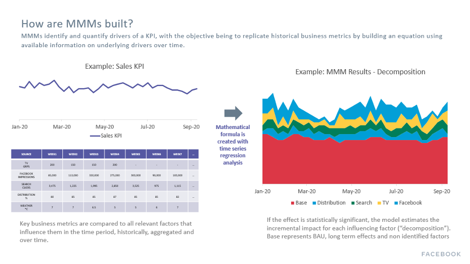
MMM is an econometric model that aims to quantify the incremental impact of marketing and non-marketing activities on a pre-defined KPI (like sales or website visits). This is a holistic model used to understand how to allocate a marketing budget across marketing channels, products and regions and can help forecast the impact of future events or campaigns:

Think about MMM as unbaking a cake. Imagine you go to a restaurant and order dessert, the cake is delicious. You want to find out what ingredients went into the cake so you can make it on your own. You find out the recipe and are good to go! You can now successfully recreate this dessert any time you want, and you may want to experiment with the recipe and see if it's successful with other ingredients, or what ratio of ingredients produces even better tasty results.

MMM is like this. It allows us to better understand the factors (ingredients) that affect business KPI (the cake) over time, allowing for flexibility.

MMMs have been around for many years and are now being rediscovered by the industry. The main reasons for this include:

• Privacy-friendly and signal-resilient - one of the key strengths of MMM is it overcomes signal loss. Other models such as multi-touch attribution are very reliant on online signals, whereas MMM does not need user level data and instead it runs off aggregated data (such as campaign level) data.
• Holistic - MMM is the established measurement solution for holistic, cross-channel sales measurement. It measures sales outcomes for all marketing channels together in one analysis. MMM accounts for the impact of both marketing (online and offline) and non-marketing activities (such as price, promotion, seasonality and distribution) on outcomes.
• Flexible - MMM is a flexible model and is adjustable based on business type (e.g. gaming, digital native, pure e-commerce, etc.) and business KPI (e.g. revenue, units sold, website activity, etc.)

How does an MMM actually work?

There are several steps within MMM. A high level view of flow of information within a MMM looks like this:

External factors and marketing inputs →	Impression and business metrics →	MMM statistical regression analysis →	Data outputs

Exact MMM methods vary by locale, vertical and company. MMM relies on regression modeling and it derives an equation that describes the KPI. This equation shows what a change in each variable means for the KPI. A series of independent variables that are expected to impact sales are used to predict the dependent variable (sales volume over time).

When running an MMM study, there are multiple steps involved. See below for the steps and approximate timings - note that these are typical timings for when you run the first study and that this can be shortened for refresh models and/or the method of implementation (e.g. in-house vs. partner):

Step	Description	Approximate Timings
Define business questions and scope	As with any research or analysis, it’s important to define the objective and key business questions that you want to be answered by the study. This will help shape how the MMM will be designed and executed, which in turn will help you get the best value out of an MMM. More details about this are in the Collecting Measurement Business Questions section section.	1-2 weeks
Data collection	Data collection is one of the most important but time consuming steps in an MMM study. Time-series data for sales (or another KPI), media, non-media marketing (e.g. promotions) and macroeconomic factors will need to be collected, cleaned and processed for MMM use. Collecting accurate and quality data is critical - if inaccurate or poor quality data inputs are used in an MMM, it will produce inaccurate and poor quality data outputs. More details about this step are in the Data Collection section.	4-6 weeks
Data review	In addition to data collection, data review is one of the most important steps in an MMM study. This involves thoroughly checking all the cleaned and processed data sets for its accuracy, just before modeling begins. Data review may also uncover data gaps or errors, which may require more data collection. As mentioned above, the repercussions of inaccurate or poor quality data inputs means inaccurate and poor quality data outputs. More details about this step are in the Data Review section.	1-2 weeks
Modeling	Once happy with the accuracy of all data inputs, the next step is to run the models. Expect modeling to be an iterative process - that is, consistently re-running and fine-tuning the models. The time and effort of this step will significantly vary based on the scope and complexity. More details about this step are in the Modeling Phase section.	4-8 weeks (dependent on MMM scope)
Analysis and recommendations	Once happy with the model, the next step is to analyse the data outputs and results and make actionable recommendations based on the original business questions in scope. There are a wide range of different outputs and metrics that come out of an MMM - more details about this step are in the Applications of the Model section.	2-4 weeks

What are the MMM options? (e.g. DIY, SaaS, 3P)

If you’ve discovered that MMM is suitable for your business - congratulations!

There are three widely accepted methods to implement a MMM. At Meta, we support all advertisers who run MMMs, no matter how you choose to run them. There are three popular ways to get started, each with varying levels of cost and resource trade-offs:

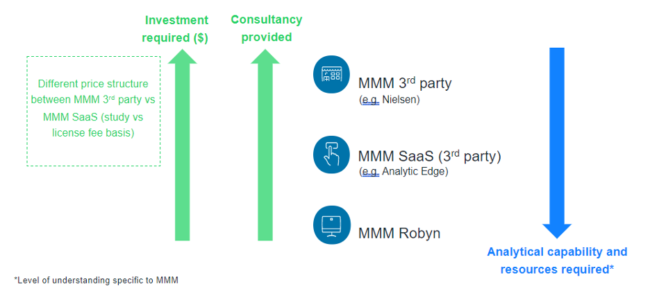
1. Working with a 3rd party MMM vendor: There are 3rd party vendors that specialise in MMMs, who usually drive the entire engagement including discovery, data collection, modeling and insights/recommendations. Most offer software that an MMM can be loaded into for forward looking simulation/optimization and forecasting capabilities.

• Pros: Offers an end to end service, requires the least amount of your time and effort (when compared to other options), can compare your MMM results with benchmarks (depending on the vendor);
• Cons: Vendor will charge a fee, usually the most expensive option when compared to other options.

How can Meta help?

Meta has preferred 3rd party MMM partners who are part of the Meta MMM Preferred Partner Program, where they have a fully vetted MMM methodology as verified by our Marketing Science MMM partnership team. You can find the full list of badged partners on our Measurement Partner website.

2. Using semi-automated MMM tools or software as a service (Saas) platforms: This new technology allows MMMs to be built in a point and click environment with less specialized MMM statistical knowledge required. MMM SaaS solutions offer automated modeling techniques that can be run on an ongoing basis and typically contain optimization planning and simulation modules for forward facing scenario planning.

• Pros: Suitable for those with less specialised MMM or analytical expertise, cheaper alternative to working with an MMM vendor;
• Cons: Less consultation than working with an MMM vendor.

How can Meta help?

Similar to 3rd party specialist MMM vendors, we also have preferred partners that offer MMM SaaS solutions - the full list of partners can be found on our Measurement Partner website.

3. Build an in-house MMM solution: For businesses who want to fully run and manage everything internally, there is the option of building an in-house MMM solution.

• Pros: Aside from headcount and time, no ongoing costs to run MMM;
• Cons: Requires in-house analytical / data science capabilities, takes the most internal time and resource investment out of all options.

How can Meta help?

The Meta Marketing Science team has built Project Robyn, an open-source R code that uses machine learning techniques for in-house and DIY modelers that clients can use to build in-house models. The code, along with detailed documentation and step-by-step guides, is available on GitHub and on this website.

Collecting your measurement business questions

When starting on your MMM journey, it’s important to collect all the business questions that you want to answer through measurement. MMM more broadly might not be the best solution to answer every question - it might actually be an incrementality study (e.g. Conversion or Brand Lift), attribution, or something else. Once collated, the right measurement solution can then be mapped to each question.

Some common questions that are best answered by MMM include:

1. How much sales (online and offline) did each media channel drive?
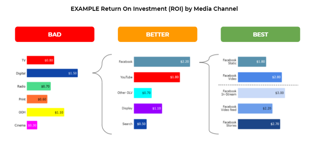
2. What was the ROI of each marketing channel?
3. How should I allocate budget by channel so as to maximize my KPIs?
4. Where should my next marketing dollar go?
5. What is the optimal level of spend for each major marketing channel?
6. How would sales be impacted if I made X change to my marketing plan?
7. If I needed to cut my marketing budget by X%, where should the dollars come from?
8. How is performance of channels such as FB impacted by the way they are executed (e.g., buying objective, frequency, creative quality or targeting strategy used)?
9. Should we raise our prices? If so, by how much?
10. What is the impact of competitor advertising on the performance of our brands?
11. How much incremental revenue to trade and promotional activities drive?

For those questions and hypotheses that are best answered by MMM, this will influence and determine the input variables and model structure. For example - if an advertiser wants to answer question #3 above, then granular data at the executional or creative level will need to be collected and used as an input in the model (more on this later). Hence this is a very important upfront step to ensure that you will get the most value out of your MMM.

Pre-Modeling Phase

---

Data Collection

Once you’ve collected all your business questions and understand which ones will be specifically answered by MMM, it’s time to get started on data collection. Data collection is one of the most important but time consuming steps in an MMM study. Collecting accurate and quality data is critical - if inaccurate or poor quality data inputs are used in an MMM, it will produce inaccurate and poor quality data outputs. Furthermore, it can be difficult collecting data in the same format across multiple different sources, making it the most time consuming step - allocate at least 4 weeks for data collection.

There are multiple factors that need to be considered when it comes to data collection.

1. Actual vs. Planned Data: It is important to aim to prioritise collecting and modeling data of events that actually occurred, instead of data of planned events. For example, aim to collect actual Facebook impressions and spends, instead of using planned Facebook impressions and spends that may have been specified in a media plan. This is because planned data may not always reflect actual occurrences and so including planned data may result in inaccurate data inputs and hence data outputs. That said, actual data may not always be available and will depend on how activities are tracked. In this instance, it may be acceptable to use planned data in the absence of actual data. A common example is Out Of Home data - because it has been historically difficult to track actual exposures, planned reach or spends can be used.

2. Dependent vs. Independent Variables: In terms of what data sets to collect, it’s important to distinguish between and determine the dependent and independent variables to be measured in the MMM:

• Dependent variable: This will be the primary KPI / metric that the MMM will measure against. The most commonly used data for the dependent variable is sales, although different data can be used depending on the vertical (e.g. account sign-ups for a telco business, home loan applications for a bank).
  • When picking which data set to use as the dependent variable, ask yourself: What is the most important KPI / metric to your business and financial report?
• Independent variables: These will be the variables or factors to be included in the MMM that should have an impact on the dependent variable. The most commonly used data sets for independent variables include media, non-media marketing (e.g. promotions, discounts), seasonality (e.g. weather, holidays) and macroeconomic factors (e.g. economic growth).
  • When picking which data sets to use as independent variables, ask yourself: What are all the different factors that have an influence on the dependent variable? Ideally we want to include everything, although this will depend on whether time series data is available for that factor.

3. What metrics should be collected?: As mentioned above, the metric collected for the dependent variable will depend on what is the most important KPI to your business. Value or volume sales are the most commonly used, but this can vary across different verticals.

For the independent variables, this will depend on the type of activity:

• Media activity: Data collected for media ideally should reflect how many “eyeballs” have seen or been exposed to the media (e.g. impressions, GRPs). Spends should also be collected in order to calculate Return On Investment, however it is best practice to use exposure metrics as direct inputs into the model, as this is a better representation than spends of how media activity has been consumed by consumers. For example, 1 dollar spent on TV might yield a different reach than 1 dollar spent on Facebook.
  • For digital activity, the most commonly used metrics are impressions. Avoid using clicks, as clicks do not account for view through conversions, and it is just as likely that someone can view an ad and convert.
  • For TV and radio, the most commonly used metrics are Gross Rating Points (GRPs) or Target Audience Rating Points (TARPs).
  • For print (e.g. newspapers or magazines), the most commonly used metrics are readership.
  • As mentioned above, aim to collect data that reflects “eyeballs” or impressions for all other channels.

Paid vs. organic?

Historically it was best practice to collect and model data for paid activity only, as this would produce more actionable results (given that it is difficult to control organic activity). However with more options to interact with consumers with organic content (e.g. branded content on Facebook), there could be good reasons to include it in the model. Robyn allows for the modeling of organic activity. More details on how to include it are here.

• Non-media marketing activity (e.g. promotions, discounts): Commonly used metrics include time-series pricing data or the use of dummy variables to indicate promotions. If it is required to measure each type of promotion separately (e.g. buy one get one free vs. gift with purchase), ensure separate dummy variables are created for each promotion.
• Seasonality and holidays: External factors that have a big impact on the dependent variable, such as seasonality and holidays, should be included in the model. There are two options for including this in the model:
  • Prophet is a Meta open source code for forecasting time series data, and has been included in the Robyn code to decompose the time series data into trends, seasonality and holidays. As Prophet automatically calculates the impact of seasonality and holidays, this is a good option for non-experts - more details on Prophet are available in the Feature Engineering section.
  • Alternatively, you can collect data for seasonality and holidays using external data sources. This will depend on how seasonality impacts your business - for example, businesses that experience fluctuation:
    • Throughout the seasons (e.g. summer vs. winter), temperature is commonly used. For key periods or specific events (e.g. Christmas, government policy change that impacts sales), dummy variables are commonly used. Similar to above, ensure separate dummy variables are created if it is required to measure each specific event separately.
• Macroeconomic factors: While this will depend on how these factors impact your business, commonly used metrics and data sets include GDP growth, unemployment, inflation.

4. How far back?: In order to get robust results, an MMM will need a minimum of two years of historical weekly data. If monthly data is only available, then it is strongly recommended to collect more than two years (e.g. 4-5 years) in order to increase the number of data points for the model.

In the ideal world, the more data the better, as this will give the model more data points to robustly capture the impact of seasonality on business outcomes.

5. How granular should the data be collected?: There are significant benefits and advantages to collecting more granular data and modeling at a more granular level. In their whitepaper, MMM vendor Ekimetrics discovered that in 75% of cases, MMMs were improved when they modelled Facebook at a more granular level by including campaign attributes.

The benefits of collecting data and modeling at a more granular level include:

• More accurate models: In the Ekimetrics whitepaper, there were improvements in the MMMs’ model fit statistics when Facebook was modelled at a more granular level. By going more granular, the model can more accurately pick up the difference in effectiveness and its impact on the dependent variable for each modelled tactic.
  • For example, separately modeling brand vs. performance activity’s impact on sales can allow the model to calculate the impact of both more accurately, where we would expect performance activity to have more of an impact on sales than brand. Alternatively, if modeling all together, the model will likely calculate the average impact of both brand and performance on sales, resulting in less accuracy.
• More actionable results: modeling at a more granular level can lead to producing results that are more actionable.
  • For example, grouping all digital activity together and modeling as total digital will produce results at the total level. Given each digital platform can operate very differently to each other, having results at the total level can make it difficult to understand what to do next. Alternatively, modeling Facebook from other digital platforms will produce separate results, which will allow for more actionable insights and next steps.

However, it is not always possible to collect granular data and model at a more granular level:

• Data availability: Granular data is not always available, where this is dependent on the data source. For most media channels and especially digital, granular data is usually available, although you will need to check how these channels are being tracked.
  • Granular Facebook data can be accessed via Meta’s MMM data UI - more details on this later. Outside of media data, this will depend on who and how the data is being collected.
  • For data that is collected internally (e.g. promotional data), this is usually available at some level of granularity, although this will depend on what the data set is.
  • For data that is collected from external data sources (e.g. macroeconomic data, weather), there is usually less flexibility on granularity as expected.
• Data variation/volume: In general, there are two factors that need to be considered in order for the model to get a robust read on a data set:
  • Variation: As regression modeling looks at the correlation between the dependent and independent variables, there needs to be some variation in the data. For example, if there is a weekly variation in sales but TV activity has remained constant for the whole time period, the model can have difficulty determining how TV has impacted sales.
  • Volume: There also needs to be a sufficient volume of observations for the model to calculate a robust result. A good way to sense check this is to ask yourself whether the activity with the low number of observations would be able to have a big enough impact on the dependent variable. For example, if there was a small amount of sampling activity in one DMA, do we expect this to have an impact on overall sales? If not, then it will be unlikely that the model is able to calculate its impact on sales.

If a data set does not have sufficient variation and volume, then it is likely that it will be better to exclude this from the model. Including more variables than necessary can lead to model overspecification (see Model Design part in Feature Engineering section), which can create noise and more difficulty for the model to accurately and robustly calculate impact. If there is a strong hypothesis that an activity has an impact on the dependent variable but the collected data doesn’t exactly meet the variation and volume test, you can try running the model with and without the activity and assess whether its beneficial to include in the model by assessing the model fit statistics (see Interpreting Marketing Mix Models output part in Applications of the model section).

There are multiple ways to think about data granularity:

• Time: Aim to collect data at the weekly level as best practice. Daily data can also be acceptable, however this would require extra data validations. The reason for this is that daily data can have more variation and hence better accuracy and more flexibility in modeling when implemented successfully, however this does come with a risk of increased noise in the model.
• Market: Aim to collect data at the DMA/state level as best practice, as there may be DMA/state level nuances that need to be accounted for. For example, coastal states in the US can have different consumer behaviours when compared to other US states. National data can also be acceptable if DMA/state level data is not available, however sense check whether there are any specific DMA/state level consumer behaviours or marketing activity that warrants a more granular model.
• Brand/Business Unit: This refers to how many separate models should be run, where a common way to break out is by brand or business unit. For example, automotive advertisers often run separate models for each car model, given that separate marketing activity is frequently run for each model and it would make less sense to run one model for all car models combined. There is no right or wrong way on how to break out by brand or business unit, however a good rule of thumb is to consider how your business makes decisions and would respond to results. For example, if separate media plans and marketing budgets are made for different financial services products like home loans and credit cards, then it makes sense to run these as separate models.
• Independent variable granularity: It is also possible to collect and model more granular data for the independent variables. For example, all digital activity historically was often combined and modelled as one variable given that it was a low proportion of total media spend. That said, digital is significantly more fragmented and complicated today and it should be broken out as best practice (see below).

At the very minimum, digital should be broken out at the channel/publisher level, given how differently each of these operate and perform (e.g. social vs. search vs. display). It is even better practice to go more granular within certain channels, where this will depend on whether there are specific business questions about this e.g. does Facebook static perform differently to video?

Even if super granular data (e.g. at the creative level) might not be collected and used in the final model, it can be a good idea to collect some of this information to help contextualise the results later. For example, a direct output from the model may be that Facebook had an ROI of $2, but there won’t be any further outputs that may explain why it was $2. Having additional details on the Facebook media and creative executions can helpful to deep dive further into Facebook’s performance, where scorecards can be built to proactively assess the quality of media and creative executions ahead of receiving the results.

How to get started?

Based on all the considerations above, a great place to start is to begin mapping out all the different variables that we want to include in the MMM. Specifying this up front can help from a project management perspective, by clearly outlining the data required and who is responsible for collecting each data set.

To help with this:

• Consider creating a trend line chart of the dependent variable - look at any big peaks or troughs and try to understand what specific activities or events drove those peaks and troughs.
• Creating a data schema can be a simple but helpful way to visualise this - see below for an example, where the specific variables will vary for every business and vertical:

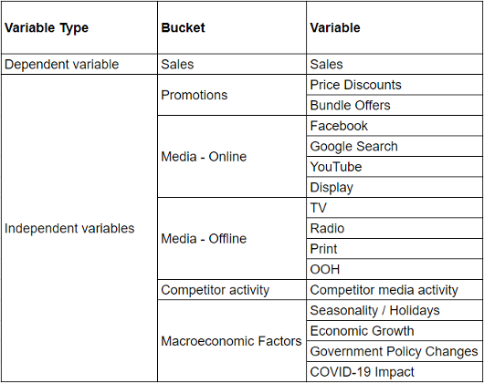
Once this has been specified, a data collection template can be used and shared with relevant stakeholders.

Meta MMM Feed: To help with Meta’s data collection, you can leverage the official Meta MMM Feed, the single source of truth when it comes to Meta MMM data. The MMM feed provides the most accurate and standardised core metrics with deeper dimensions and granularity for optimal MMM workflows. It provides impression and spend data in a consistent and easy to use format for the creation of MMM variables. The data contains granularity and can be split by day, country, region, placement, objective, format, campaign and ad set.

Vendors through the Preferred Partner Program should already have access to the Meta MMM Feed with the self-serve user interface. To access the Feed via a non-badged 3rd party or with in-house modeling, reach out to your Meta representative.

Additional Data Collection Tips: Based on previous experiences, see below for some tips to help make data collection easier:

• Collect media or marketing plans: While these shouldn’t be used as data inputs, they are an invaluable source of information. Plans can help clarify what data needs to be collected and check whether the collected data is accurate.
• Start with a data sample: Instead of collecting the full data set for the whole time period, collect a data sample (e.g. a few months of data) to check if it’s in the correct and desired format. While this could be more work than necessary, the extra diligence can potentially save time and effort later down the track and prevent having to re-pull data.
• Clarify the starting day for weekly models: If running weekly models, clarify up front what day the data starts on e.g. week commencing Sundays vs. Mondays. Again, this can potentially save a lot of time and effort later down the track if all parties are aligned on the same approach

Data Review

Once all data has been collected, a data review should be conducted to review it for its accuracy and whether it aligns with the media plan, expectations and if it can answer the desired business questions.

Along with data collection, data review is one of the most critical stages in an MMM study. If the collected data is not reviewed, ends up being inaccurate and is used in the MMM, then the data outputs will also be inaccurate and not reliable - hence the common saying “rubbish in, rubbish out”.

How to run a data review?

Reviewing many different time-series data sets for its accuracy can be a difficult and time-consuming process. There is no right or wrong way to run a data review - checking the data very thoroughly at the most granular level can give the most confidence, but it can be the most time consuming. That said, checking the data at a topline level can be very quick, but it might not establish the most confidence.

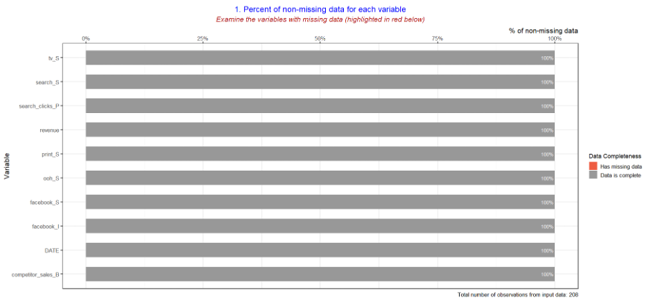
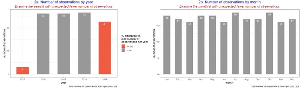
Below is an example of data review charts you can consider producing for data review (These charts are not included in the current Robyn code)

• The following charts provide descriptive statistics or a basic overview of the collected data inputs. They will be useful to help determine if there is any missing or incomplete data and can help identify the specific variable (e.g. media channel) that requires further investigation.

• The following charts help analyse the correlation between all the different variables:
  • Chart 3a specifically looks at the correlation between each independent variable and each other. This can be useful to help determine multicollinearity, which occurs when two or more independent variables are highly correlated with each other. Multicollinearity can be problematic for a regression model, as the model can experience difficulty calculating the impact of each of the different independent variables, especially if they are all highly correlated with each other. In turn, this can help decide which variables to include in the final model.

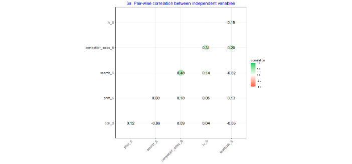
• Alternatively, chart 3b looks at the correlation between each independent variable with the dependent variable. This can help visualise whether there is an expected impact between an independent variable and the dependent variable and can be useful to determine whether a specific independent variable should be included or not.

• The following charts will be most useful to help check for the accuracy of the collected data. Use charts 4 and 5 to sense checks against media plans or with another person who is closer to the media activity, which can be a useful way to establish confidence in the collected data. In addition, if certain business questions require more granular data, it is important to check that the collected data is granular enough to measure and answer the question.

Ultimately at the end of the data review process, we want to feel confident that all the collected data is clean and accurate and so the data outputs can be trusted as accurate.

Modeling Phase

---

If you have successfully collected and reviewed the data required for modeling based on the guide from previous sections, congratulations! You can assume that you are approximately halfway through your Robyn journey. While data collection and review is one of the most important but time consuming steps, using Robyn means that you can now benefit from its core features without developing them by yourself. Robyn provides end-to-end scripts for modeling, which can be taken as a whole or in part to empower other MMM projects. If your data inputs are ready to go and in the required template and you follow the step by step demo script, you can complete the modeling phase. While Robyn aims to increase automation and minimize human bias, it does not mean that it can successfully run without any intervention. Rather, analysts still need to play a very important role by fine-tuning parameters, executing different modeling techniques, and interpreting results to develop actionable recommendations that will improve marketing practices. Therefore, in this section, we will cover analyst considerations and caveats when running Marketing Mix Modeling with Robyn.

Feature Engineering

Feature engineering is the process of transforming raw data into features that better represent the underlying problem to the predictive models, resulting in improved model accuracy on unseen data (more details on feature engineering here). Today’s MMMs are more sophisticated and introduce different feature engineering techniques. Feature engineering can be as critical as data collection, as the process transforms the way raw data is informed in modeling. Therefore it is very important to understand the underlying assumptions in each technique, otherwise the result can be misleading.

Prophet Seasonality Decomposition:

Depending on the vertical, the dependent variable (e.g. sales, conversions) will likely be impacted by underlying seasonality trends. Given that Robyn and MMM uses time-series data, a time-series analysis (wiki) can be used to determine the seasonality trends which in turn can be incorporated in the final model.

Prophet is a Meta open source code for forecasting time series data. Prophet has automatically been included in the Robyn code to decompose the data into trend, seasonality, holiday and weekday impacts, in order to improve the model fit and ability to forecast. Traditionally it would be required to collect and model seasonality and holiday data as separate dummy variables in the model. However, Prophet makes this process much easier, especially for those new to Robyn and MMM. In the Robyn code, analysts can simply add time series baselines with Prophet. If you are not clear on which baselines need to be included in modeling, please refer to the following description:

• Trend: Long-term and slowly evolving movement (either increasing or decreasing direction) over time. In marketing, the trend can be generated by factors which can create long-term momentum (e.g. general market growth in specific categories, gradual economic downturn, etc.)
• Seasonality: The repeating behavior that can be captured in a short-term cycle, usually yearly. For example - depending on the vertical or category, specific brands can have more sales in summer than winter.
• Weekday: The repeating behavior that can be captured within a week. Note that this is only usable when daily data is available.
• Holiday/Event: Holidays or other events that highly impact your dependent variable. (e.g. national holiday, mega sales day, etc.)

If you do not already have trend/seasonality data of your own, we would recommend you consider using Prophet for at least the trend and seasonality components. However as the complexity of the model and industry being measured increases, it may be worthwhile exploring additional ways to account for time-based trends e.g. collecting other data sources.

Pro-tip: Customize holiday & event information

You can use a built-in collection of country-specific holidays from the default “dt_holidays'' Prophet file. This file includes national holidays for 59 countries and you may review the list by running: data("dt_prophet_holidays"). However this information might not perfectly align with your business calendar. For example, eCommerce businesses can have a revenue impact several days prior to holiday as items need to be delivered before holiday. Alternatively another business might have a unique mega sales day, independent of the national calendar. In this case, you can try following:

• Customize holiday dataset: You can consider changing the information in the existing holiday dataset, in case your business has carry-over or prior impact. In addition, any type of events (not just holidays) can be added into this table e.g. school holidays, Black Friday, Cyber Monday, etc.
• Add an additional context variable: If you use the ‘holiday’ information from Prophet, all the various holidays/events will be aggregated and modelled as one variable. If you need to measure the impact of a specific day or event as a separate variable, consider adding that information into context_vars. In this case, make sure that you do not provide duplicate information across the two sources (i.e. Prophet holiday and additional column). Alternatively, if good quality data has been collected to explain certain different holidays and events, this can be modelled as a specific independent variable and turn off the holiday option in Prophet.

Model Window

As MMM models are built on historical data, an important consideration is selecting the right time period to specifically use for modeling from the historical data collected. There are pros and cons of using a longer vs. shorter time period:

• The advantage of a rolling window is that you may still use the full data history (e.g. 4 years) to more accurately determine the trend, seasonality and holiday effects.
• Alternatively, defining a specific range (e.g. 18 months) for media, organic and contextual variables can be a better option as it more accurately reflects your current business and marketing scenarios.

Fortunately you can achieve this balance with the model window feature in Robyn. For example, with Robyn's integrated dataset of 208 weeks, users can set the ‘modeling period’ to a subset of available data (e.g. 100 weeks), while the trend/seasonality/holiday variables are still derived from the entire 208 weeks, which improves the accuracy for time-series decomposition.

When it comes to choosing a modeling window, this is not a simple question to answer. This will vary depending on each business and dataset - see below for some general considerations to help with choosing:

• Business context

  Business context is always important and should be considered. Analysts should ask themselves ‘how much time is enough to capture recency in modeling and also deliver up-to-date results?’ Factors such as internal shifts in marketing practices, ad platform evolvement, external macro factors should be considered. As addressed in the Data Review section, charting data is always helpful to visualise.

• Data sparsity

  Data sparsity also needs to be considered. There must be balance so that there are enough data points captured in the modeling window. The recommended ratio of data points is 1 independent variable : 10 observations. For example if you aim to run a model with recent 6 month data, weekly data will be too sparse to fit the model and so daily data is recommended in this case. If your dataset is not long enough to split the model window, you can simply start fitting the model with the entire period you have.

Ultimately if you are not sure about which model window to use, don’t stress! Experiment with several different windows as part of an iterative process.

Model Design

Designing a model is a balance between answering all the specified business questions and correctly specifying the model. Model overspecification occurs when too many independent variables have been included in a model and the model produces one or more redundant predictor variables. That is, the model has difficulty in accurately calculating the coefficient or impact of one or more independent variables on the dependent variable.

Using a table like the below can be valuable to help articulate how the model will be built:

Once you have designed your model, you will need to tell Robyn how you designed the model by configuring a couple of parameters in the code:

• Control the signs of coefficients: If you put the ‘default’ sign on the coefficient setting in Robyn, the respective variable could have either positive or negative coefficients depending on the modeling result. However, sometimes it makes sense to assume that an independent variable will have a specific impact on the dependent variable e.g. competitor sales should have a negative impact on one’s sales or an advertiser’s media activity should have a positive impact on one’s sales. In this case, you can directly control the sign of coefficients in the parameter setting to be either ‘positive’ or ‘negative’.
• Categorize variables into Paid Media, Organic and Context variables: There are three types of input variables in Robyn i.e. paid media, organic and context variables. Check below for general considerations on how to categorise each variable into these three buckets:
  • paid_media_vars: Any media variables with a clear marketing spend falls into this category. Transformation techniques will be applied to paid media variables to reflect carryover effects (i.e. adstock) and saturation (see the Data Transformation Techniques section for more details). For these variables, it is recommended to use metrics that better reflect media exposures such as impressions, clicks or GRPs instead of spend. If not available, spends can be used as a last resort.
  • organic_vars: Any marketing activities without a clear marketing spend fall into this category. Typically this may include newsletters, push notifications, social media posts, etc. As organic variables are expected to have similar carryover (adstock) and saturating behavior as paid media variables, similar transformation techniques will be also applied to organic variables.
  • context_vars: These include other variables that are not paid or organic media that can help explain the dependent variable. The most common examples of context variables include competitor activity, price & promotional activity, macroeconomic factors like unemployment rate, etc. These variables will not undergo any transformation techniques and are expected to have a direct impact on dependent variables.
  • Note: organic_vars and context_vars can accept either categorical or continuous data, while paid_media_vars can only accept continuous data. If there are organic or context variables which are categorical, you will need to specify which variables are categorical in the factor_vars parameter. Also keep in mind that for the same variable, continuous data can provide more information to the model than categorical. For example, specifying the discount % of each promotion (which is continuous data) will provide more accurate information to the model vs. a dummy variable that indicates the presence of a promotion with 0 and 1.
• Impression vs. Spend:

  As addressed in the Data Collection section, it is recommended to use media exposure metrics like impressions or GRPs for modeling. While it isn’t recommended to use for modeling purposes, media spends should also be collected in order to calculate a Return On Investment (ROI) and to help simulate budget allocations. When using exposure variables like impressions instead of spend in paid_media_vars, Robyn fits a nonlinear model with Michaelis Menten function between exposure and spend to establish the spend-exposure relationship (more details are available on the official Robyn github page - search for ‘Spend exposure plot’). Therefore you don’t need to worry about the process of converting exposure back to spending at the end. Although using exposure metrics is best practice, there can be some situations where spends have to be used for modeling purposes:

  • Media exposure metrics are available to be collected;
  • The impression and spend data is a poor fit in the model - for example, a large advertiser having multiple teams using different strategies (bidding, objective, audience etc.) for Facebook ads. Because of this fragmentation, it is possible that impression and spend data at the total Facebook level will fit poorly - Robyn will produce a warning message when impressions and spends do not fit well. In this situation, the first step you should consider is to split Facebook into meaningful variables. However, if it is not feasible to achieve more granularity or if the impression and spend data still fits poorly even after trying all possible splitting options, you may consider using spend instead of impressions.

• Finalize by considering the number of input variables: Fortunately Ridge regressions in Robyn (covered in a later section) deals with intercorrelated explanatory variables and prevents overfitting. Therefore, analysts can have more flexibility when choosing which variables to include. Generally it is recommended to use the following rule of thumb when finalizing the number of input variables - for an n * p data-frame (where n = num of rows to be modelled and p = num of columns), n should be about 7-10x more than p where we recommend going no more than 10x. If unsure, it is worthwhile to try multiple designs as part of an iterative process.

Data Transformation Techniques

Part of MMM’s appeal is that it is grounded in key marketing principles, such as adstock and saturation, where these principles are further reflected in Robyn:

• Adstock: This technique is very useful for a better and more accurate representation of the real carryover effect of marketing campaigns. Moreover, it helps us understand the decay effects and how this can be used in campaign planning. Adstock reflects the theory that the effects of advertising can lag and decay following an initial exposure. In other words, not all effects of advertising are felt immediately - memory builds and people sometimes delay action until following weeks, where this awareness diminishes over time.
• Saturation: The theory of saturation entails that each additional unit of advertising exposure increases the response, but at a declining rate. This is a key marketing principle that is reflected in MMM and Robyn as a variable transformation.

You can find more technical details on both of these here, including the underlying equations. It is important that you understand the meaning of each hyperparameter correctly before fine-tuning and adjusting it - if unsure, you can simply use our recommended settings as described below.

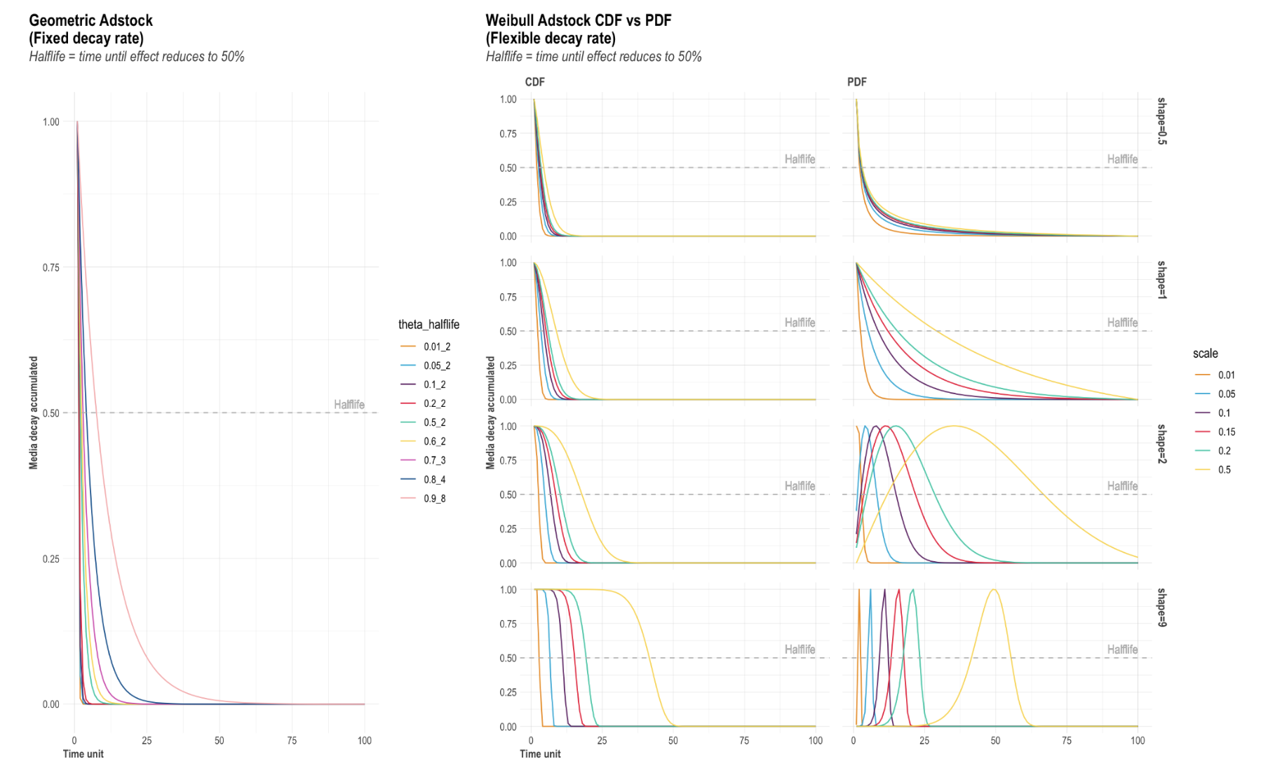
Adstock

There are two adstock techniques you may choose from in Robyn, each with its pros and cons. In order to find the approach that best fits your model objectives and business purposes, we recommend testing various transformations.

1. Geometric - the biggest advantage of the Geometric transformation is its simplicity. It only requires one parameter called ‘theta’ that can be quite intuitive. For example, an ad-stock of theta = 0.75 means that 75% of the impressions in period 1 were carried over to period 2. This can make it much easier to communicate results to non-technical stakeholders. In addition, Geometric is much faster to run than Weibull, which has two parameters to optimize.

   However, Geometric can be considered as too simple and often not suitable for digital media transformations, as shown in this study. When it comes to setting hyperparameters for a Geometric transformation technique, theta is the only parameter that can be adjusted, which reflects the fixed decay rate. For example, assuming TV spend on day 1 is 100€ and theta = 0.7, then day 2 has 100x0.7=70€ worth of effect carried-over from day 1, day 3 has 70x0.7=49€ from day 2 etc. A general rule-of-thumb for common media channels are:

   • TV = c(0.3, 0.8)
   • OOH/Print/Radio = c(0.1, 0.4)
   • Digital = c(0, 0.3)

2. Weibull - while the traditional exponential adstock is very popular, it was recently reported by Ekimetrics & Annalect that the Weibull survival function / Weibull distribution can better fit modern media activity such as Facebook. The Weibull survival function / Weibull distribution provides significantly more flexibility in the shape and scale of the distribution. However, Weibull can take more time to run than Geometric, as it optimizes two parameters (i.e. shape and scale) and it can often be difficult to explain to non-technical stakeholders without charting.

When it comes to setting hyperparameters for the Weibull transformation technique, this will depend on which type of Weibull transformation:

• Weibull CDF adstock: The Cumulative Distribution Function of Weibull has two parameters - shape & scale. It also has a flexible decay rate, whereas Geometric adstock assumes a fixed decay rate.

  • The shape parameter controls the shape of the decay curve, where the recommended bound is c(0.0001, 2). Note that the larger the shape, the more S-shape and the smaller the shape, the more L-shape.
  • The scale parameter controls the inflexion point of the decay curve. We recommend a very conservative bound of c(0, 0.1), because scale can significantly increase the adstock’s half-life.

• Weibull PDF adstock: The Probability Density Function of the Weibull technique also has two parameters in shape & scale, and also has a flexible decay rate as Weibull CDF. The difference to Weibull CDF is that Weibull PDF offers lagged effects.

  For the shape parameter:

  • When shape > 2, the curve peaks after x = 0 and has NULL slope at x = 0, enabling lagged effect and sharper increase and decrease of adstock, while the scale parameter indicates the limit of the relative position of the peak at x axis;

  • When 1 < shape < 2, the curve peaks after x = 0 and has infinite positive slope at x = 0, enabling lagged effect and slower increase and decrease of adstock, while scale has the same effect as above;

  • When shape = 1, the curve peaks at x = 0 and reduces to exponential decay, while scale controls the inflexion point;

  • When 0 < shape < 1, the curve peaks at x = 0 and has increasing decay, while scale controls the inflexion point.

    While all possible shapes are relevant, we recommend c(0.0001, 10) as bounds for shape. When only strong lagged effects are of interest, we recommend c(2.0001, 10) as bound for shape.

  When it comes to scale, we recommend a conservative bound of c(0, 0.1) for scale.

Due to the great flexibility of Weibull PDF and more freedom in hyperparameter spaces for Nevergrad to explore, it also requires a large number of iterations for modeling.

If the description above is too complicated, you can access the adstock helper plot in Robyn which visualizes how the three adstock options Geometric, Weibull CDF & Weibull PDF are transforming the data as the parameter changes. See below for example charts:

Saturation

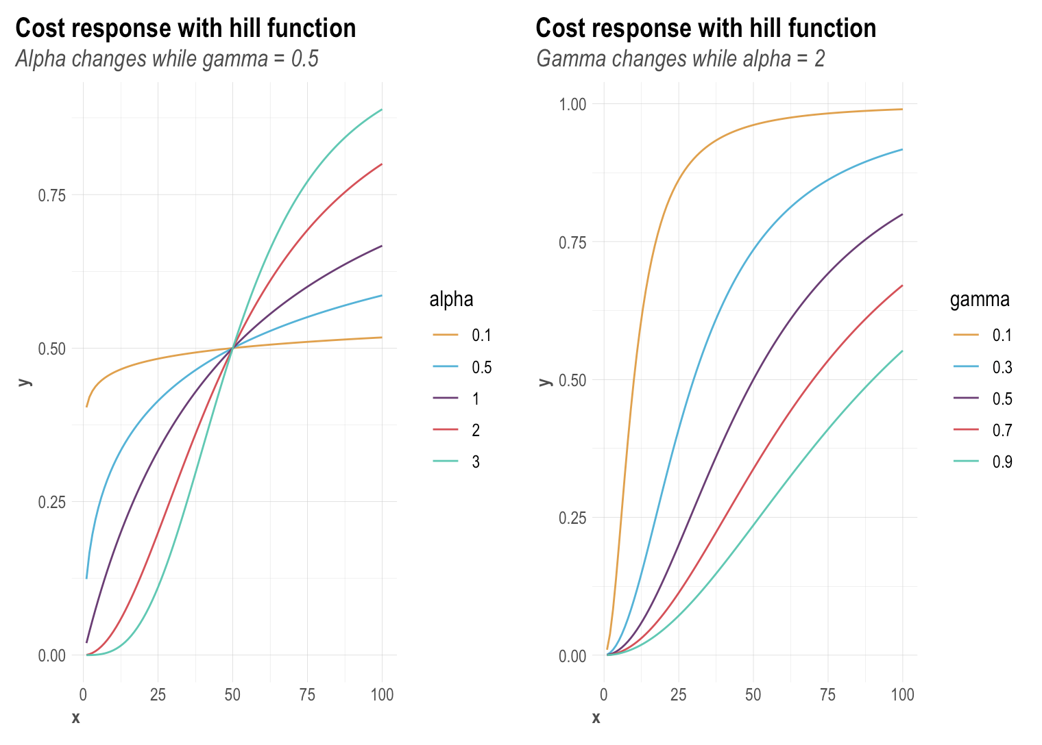
Robyn utilizes the Hill function to reflect the saturation of each media channel. A Hill function is a two-parametric function in Robyn with alpha and gamma:

• Alpha controls the shape of the curve between exponential and s-shape. We recommend a bound of c(0.5, 3) - note that the larger the alpha, the more S-shape and the smaller the alpha, the more C-shape.
• Gamma controls the inflexion point. We recommend a bound of c(0.3, 1) - note that the larger the gamma, the later the inflection point in the response curve.

You can also access the helper plot to see how the Hill function transforms as the parameter changes - see below for some example saturation charts:

Modeling Techniques ​

Once you finish setting the parameters in feature engineering, it is now time to run your first model. Fortunately once parameters have been set, Robyn’s modeling process is automated and the results will be automatically generated according to the model specification you have made. Therefore, less intervention is required in this part, however it is important to understand what is happening behind the scenes and how to interpret the results.

Ridge Regression

MMM uses regression modeling, which aims to derive an equation that describes the dependent variable. The model aims to assign a coefficient to each independent variable, where only the variables that are statistically significant stay in the model.

In very simple terms, the following model shows how the KPI is affected by changes in all the factors you have data for (you can find a more detailed equation for the Robyn model here):

KPIt = β0 + β1x1 + β2x2 + β3x3 + β4x4 + … + βnxn

• KPIt : The KPI at the time (t) you want to model.
• β0: The base performance, or what performance would be if all other factors were at their minimum.
• β: The coefficients, or what a change in the variable (x) means for the KPI.

Overfitting and multicollinearity are commonly addressed issues in regression analysis. Overfitting the model will take away from it’s predictive powers as you are taking away the flexibility with the model. On the other hand, not having enough variables and underfitting can lead to improper reads into certain channels. In order to address multicollinearity among many regressors and prevent overfitting we apply a regularization technique to reduce variance at the cost of introducing some bias. This approach tends to improve the predictive performance of MMMs.

The most common regularization and the one used in Robyn is Ridge regression - for more details on the mathematics behind it, see this page. In Robyn, Ridge regression is automatically built in and there are fortunately not many settings that you need to configure - however, if keen to configure further, refer to the tip below.

Pro-tip: control the amount of penalty in Ridge regression

*Warning: only recommended for those who have foundational understanding in regularization techniques*

Regularization technique in Ridge regression is achieved by penalizing the regression model. This means that Ridge regression will shrink coefficients towards zero if those variables have a minor contribution to the dependent variable.

You can control the amount of penalty by controlling the lambda(λ) parameter in Ridge regression. When lambda increases, the impact of the shrinkage grows, leading to a decreased variance but increased bias. In contrast, when lambda decreases, the impact of the penalty decreases, leading to increased variance but decreased bias.

Robyn is taking lambda.1se, the lambda which gives an error that gives one standard error away from the minimum error. Lambda.1se has been the rule of thumb when choosing lambda and it is the default setting in glmnet. However, sometimes the rule of thumb does not always work as intended. In that case, you can control lambda between lambda.min(less penalty) and lambda.1se from the lambda_control parameter in the robyn_run function.

Model Selection

Model selection is a core part of the modeling process in Robyn. Building MMMs manually can be a very time-consuming process because MMMs are likely to contain a high cardinality of parameters to adjust (please refer to the Data Transformation Technique section part in the Feature Engineering section). Adjusting different hyperparameters can involve many subjective decisions, modeling experience and trial and error over hundreds of iterations, where it can take months to build an MMM from scratch. Fortunately, Robyn is able to automate a large portion of the modeling process and thus reduce the time taken to run a model as well as the "analyst-bias".

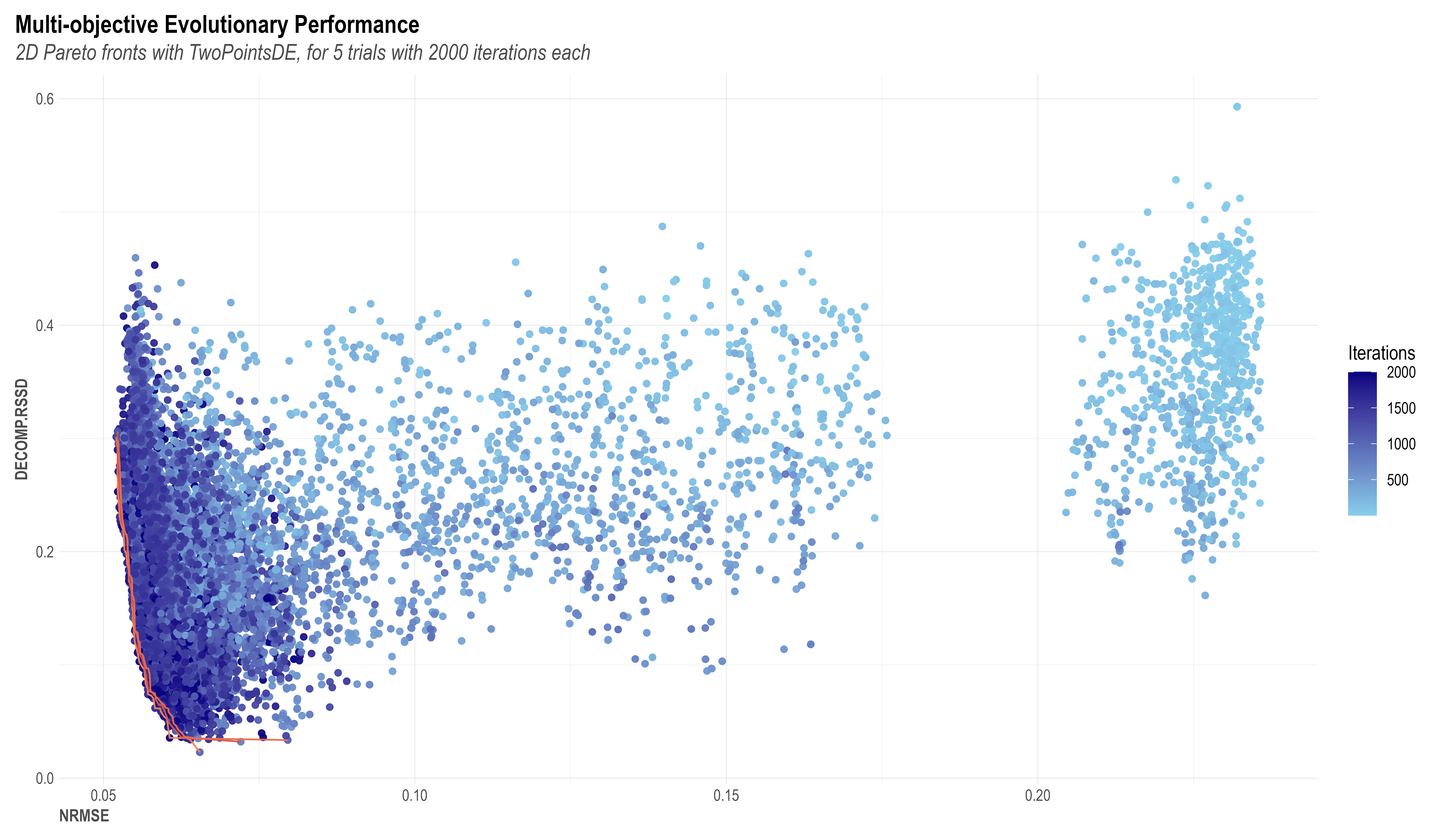
Robyn provides a semi-automated model selection process by automatically returning a set of optimal results. To accomplish this, Robyn leverages the multi-objective optimization capacity of Meta's evolutionary optimization platform Nevergrad. When exploring the best hyperparameters to select, Robyn tasks Nevergrad with achieving two objectives:

• Model fit: Aim to minimize the model’s prediction error (NRMSE or normalized root-mean-square error)
• Business fit: Aim to minimize decomposition distance (DECOMP.RSSD, decomposition root-sum-square distance). The distance accounts for a relationship between spend share and a channel’s coefficient decomposition share. If the distance is too far, its result can be too unrealistic - e.g. media activity with the smallest spending gets the largest effect.

The chart below elaborates how Nevergrad eliminates the majority of "bad models" (larger prediction error and/or unrealistic media effect). Each dot in the chart represents an explored model solution (one unit of hyperparameter sampling), while the lower-left corner lines are Pareto-fronts 1-3 and contain the best possible model results from all iterations. The two axes (NRMSE on x and DECOMP.RSSD on y) are the two objective functions to be minimized. As the iteration increases, a trend down the lower-left corner of the coordinate can be clearly observed. This is proof of Nevergrad's ability to drive the model result towards an optimal direction.

At the end of the modeling process, Robyn will generate a series of models as initial outputs based on the NRMSE & DECOMP.RSSD function. After reviewing charts and considering the user’s business knowledge and requirement, a final model should be selected by the user to continue with the next steps. You can find more information on how to interpret outputs here.

What are the best practices to select the final model among all Pareto-optimum output?Instead of automatically picking the best model, we have decided to allow users to choose the final model using pareto optimal outputs. The reasons behind this decision are two-fold:

• MMM studies are complex, where we don’t believe that a handful of statistical parameters can be used to accurately select a model that reflects the various business contexts and different companies;
• Being open source, Robyn is designed to be transparent. In turn, this means that we have chosen for Robyn to not be a black box solution and have enabled users to make the final decision in the spirit of transparency.

Below are general considerations you can refer to when selecting the final model:

• Experimental calibration: We believe integrating experimental results into MMM is the best choice for model selection. We will cover more details about this in the later section.
• Business insight parameters: You can evaluate the models by checking whether the results match your business context. There can be multiple business parameters to review e.g. ROI, media adstock and response curves, share and spend contributions, etc. If you have a strong prior knowledge of performance, such as industry benchmarks, previous MMM/MTA results, this can also be a good reference point to help you decide the final model.
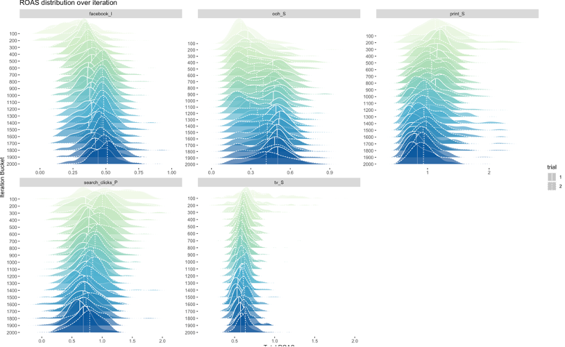
• ROAS convergence over iterations chart: The below charts can also be used to help select the model, which shows how ROI for paid media or ROAS evolves over time and iterations. For some channels, it's clear that the higher iterations are producing more "peaky" ROAS distributions, which indicated higher confidence for certain channel results.

• Statistical parameters: If multiple models show the very similar trends in business insights parameters, you can simply choose the model with best statistical parameters (e.g. the highest adjusted R-square, the lowest NRMSE, etc.)

Pro tip: Parameter setting options in Nevergrad optimization

• Number of iterations: Robyn recommends the high number of iterations (e.g. 2000 iteration x 5 trials for geometric adstock). The larger the dataset, the more iterations are required to reach convergence. However, in the situation that you would like to quickly check how the code runs, you can save time by substantially reducing the number of iterations. That said, it isn’t recommended to use and depend on these results to make business decisions.
• Number of pareto frontlines: In case you would like to have more spectrums in pareto optimal results, you can increase the number of pareto frontlines in the robyn_run function (note that the default number is three frontlines).

Model Calibration

As mentioned above, we strongly recommend using experimental and causal results that are considered to be the ground truth to calibrate MMM. People-based e.g. Meta Conversion Lift, or geo-based incrementality studies e.g. Meta GeoLift are two methodologies that can be used to establish the true incrementality of your advertising. By applying the results from these experiments, it is highly likely that this will improve the accuracy of your models.

As discussed in the Model Selection part, calibration can increase your confidence when selecting the final model, especially when there is no strong prior knowledge of media effectiveness and performance. It is recommended to run incrementality studies on an ongoing and regular basis in order to have results that can permanently calibrate the MMM. In general, we want to compare the results of an incrementality study with the MMM outputs for a marketing channel. Conceptually, this method is like a Bayesian method, where experiment results are used as a prior to calibrate the coefficients of media variables.

The figure below shows the calibration process for one MMM candidate model. Meta’s Nevergrad gradient-free optimization platform allows us to include the MAPE(cal,fb) as a third optimization score besides Normalized Root Mean Square Error (NRMSE) and decomp.RSSD ratio providing a set of Pareto optimal model solutions that minimize and converge to a set of Pareto optimal model candidates. This calibration method can be applied to other media channels which run experiments, the more channels that are calibrated, the more accurate the MMM model:

Some other tips to help with calibration:

• Ensure that the incrementality studies align with what the MMM is measuring e.g. the same level of granularity, same metrics measured, and within the same period, etc.
• Avoid using results from incrementality studies when its confidence is not high enough.
• Note that currently, Robyn only accepts point-estimate as a calibration input. For example, if $10k spend is tested against a hold-out for channel A, then input the incrementality study results as a point-estimate by specifying 1) the starting date, 2) end date, and 3) incremental response. The reason why Robyn only accepts point-estimates is that experimental incrementality studies only account for a marginal impact from a certain period, not the whole modeling window.
• Try to use a longer study duration in incrementality studies to capture long-tail conversions and to reduce bias. Longer studies might introduce noise in the result, but variance reduction techniques can help minimise this (e.g. advanced results in Meta Conversion Lift).

Model Refresh

After the initial model is built and selected, the robyn_refresh() function can be used to continuously build model refreshes when new data arrives. This capability enables MMM to be a continuous reporting tool on a regular frequency (e.g. monthly, weekly or even daily) and therefore can make MMM more actionable.

For example, when updating the initial build with 4 weeks of new data:

• robyn_refresh() uses the selected model of the initial build;
• Robyn then sets the lower and upper bounds of hyperparameters for the new build, which will be in line with the selected hyperparameters of the initial build. This will therefore stabilise the effect of contextual and organic variables across initial and new builds as well as regulating the new share of effect of media variables towards the new added period spend level;
• Once this is complete, Robyn will produce aggregated results containing the initial and new builds for reporting purposes and their corresponding plots.

The example below shows mode refreshes for 5 different periods of time, based on an initial time period covering 2017-2018:

A set of results for each refresh period will also be produced, which will include ROI and effects from each of the variables within the model. Note that the baseline variable will be the sum of all Prophet variables (e.g. trend, seasonality, weekday and holiday) plus the intercept. Based on this plot, you can get an idea of how the impact from different business levers changes over time. The charts are based on simulated data and do not have real-life implications:

Note that refreshing models might not always be the best approach, where there are some scenarios whereby it is better to rebuild the model:

• Mostly new data: If the initial model has 100 weeks and there is 80 weeks worth of new data to be added as a refresh, it might be better to rebuild the model;
• Addition of new variables: If new variables need to be added, then the model design will need to be changed and hence it is better to rebuild the model.

Applications of the Model ​

You may have heard this quote by John Wanamaker where he laments: “Half the money I spend on advertising is wasted; the trouble is I don’t know which half.” One of the benefits of MMM and Robyn is that it can measure the effectiveness of all your advertising and also provide actionable insights to improve the effectiveness of various marketing activities. To achieve this, you must be able to correctly interpret the outputs of the model. Please note that the following outputs and charts are based on simulated data and are for illustrative purposes only.

Interpret Marketing Mix Model Outputs

To enable actionable decision making, Robyn produces a range of outputs and charts like the below

Model fit: In order to have an accurate model, the fit of the modelled data has to be accurately relative to the actual data provided. As mentioned in the Model Design section, overspecifying the model will erode its predictive powers, however not having enough variables and underspecifying can lead to improper reads into certain channels. The graph below is an example of a well fit model that shows actual data compared to modelled data. In this example, the red line is the actual sales week over week, while the blue line represents the predicted sales from the model.

Modellers should strive for a high R-squared, where a common rule of thumb is

• R squared < 0.8 = not ideal, aim to improve;
• 0.8 < R squared < 0.9 = acceptable, if possible aim to improve;
• R squared > 0.9 = ideal.

Models with a low R squared values can likely be improved upon. Common ways to improve it include having a more comprehensive set of independent variables - that is, split up larger paid media channels or include additional baseline (non-media) variables that may explain the dependent variable.

Volume Contribution: In addition to being able to compare actual vs. modeled data, we can also see the incremental volume contributions from each modelled independent variable. The chart below shows an example of Facebook’s volume contributions to sales vs. all other variables that were included in this model. For example in the chart below, 2.2% for Facebook means that 2.2% of the total sales is being driven by Facebook.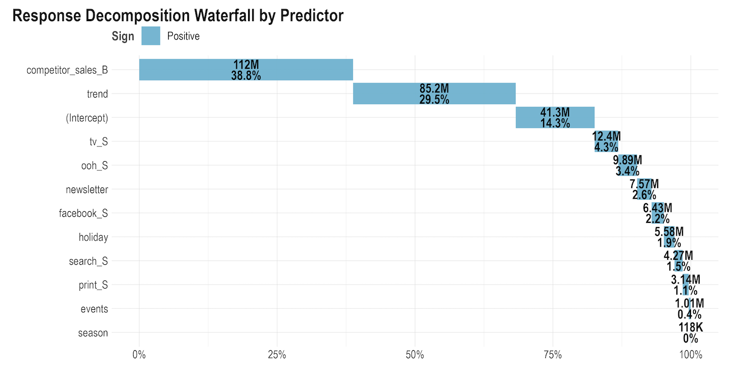Share of spend vs. effect with total ROI:

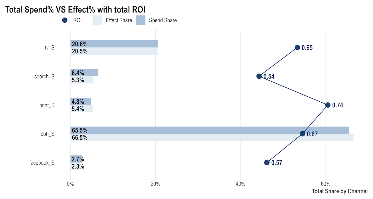
Some Robyn outputs allow us to drill down even more to get more valuable incremental insight. The chart below shows the detailed impact of media contributions by comparing and contrasting several different metrics:

• The share of spend reflects the relative spending of each channel;
• The share of effect is the same as volume contribution i.e. how much incremental sales were driven by each channel;
• ROI (Return On Investment) represents the efficiency of each channel and is calculated by taking the incremental revenue driven by a channel, divided by how much was spent on that channel.

These metrics are usually compared between other media channels over every reporting period. It’s important to consider all metrics before making decisions, as making a decision based on one data point might not reflect the whole picture. For example:

• A channel with a high ROI but low contribution and spend can indicate a potential increase in spend, given that it is delivering good returns and is likely to not be saturated due to the low spends;
• A channel with a low ROI but high contribution and spend might seem like it’s underperforming and hence spend should be moved away from it, however it is a big driver of performance and so this might not be wise. Consider looking into how to optimise this channel, given that it is an important channel.

Response curve: Sometimes called saturation curves, response curves indicate if a specific media channel’s spend is at an optimal level or if it is approaching saturation and therefore suggest potential budget reallocation. The faster the curves reach an inflection point and to a horizontal/flat slope, the quicker the media channel will saturate with each extra ($) spent. A side by side comparison of response curves for each media channel can offer insights into the best opportunities to reallocate spends from more saturated to less saturated channels to improve outcomes: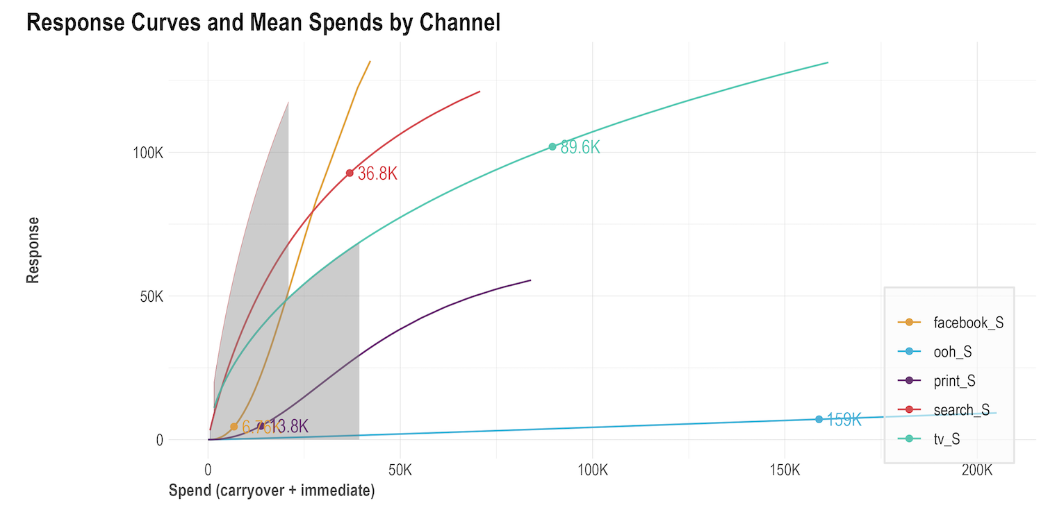Adstock decay rate: This chart represents, on average, the percentage decay rate each channel had. The higher the decay rate, the longer the effect that a specific media channel has after the initial exposure.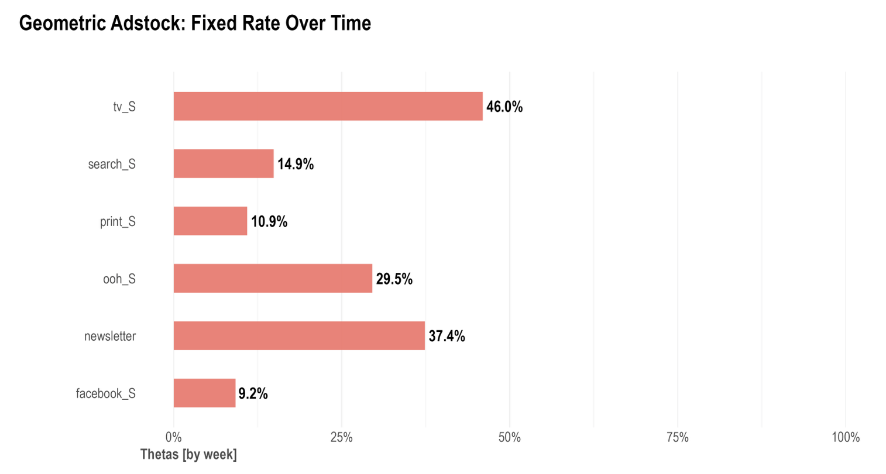Budget Allocator

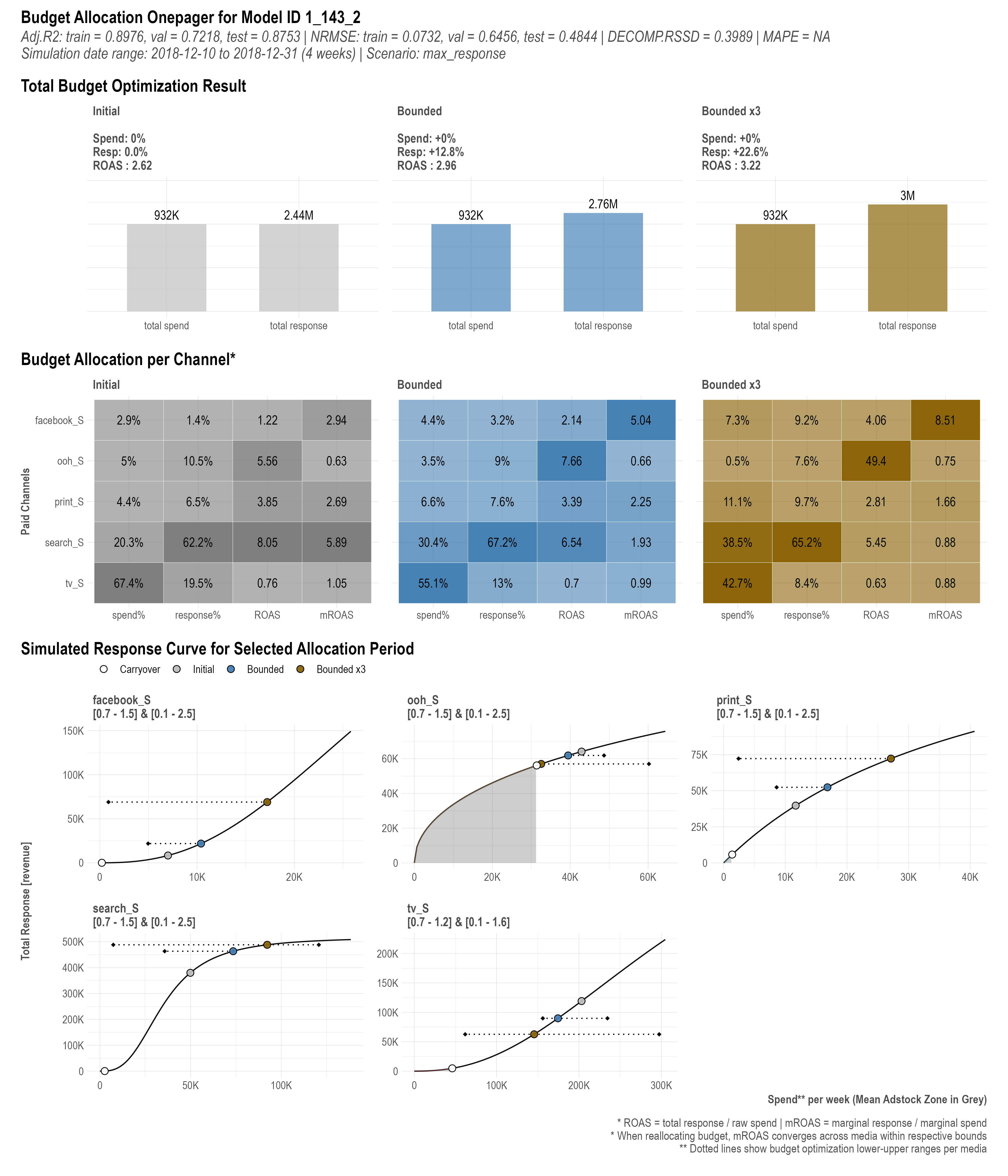
MMMs can produce a lot of outputs, which can often lead to the questions “how can I use all the results to make business decisions?” or “how can I allocate my media budgets based on the multiple results such as volume contribution, ROI, and response curve?” Indeed, finding an optimal budget allocation based on MMM outputs can be challenging. Fortunately, Robyn offers a built-in budget allocator function which uses all the model results to simulate and predict different budget allocations, which in turn enables actionable decision making.

Even though the code has been thoroughly reviewed by Meta and the Robyn community, we don't guarantee that using Budget Allocator as well as any Robyn's functions will meet business expectations on predicted response's accuracy. Please consider validating outputs before the implementation.

For every selected model result, the robyn_allocator() function can be applied to get the optimal budget mix that maximizes the response. There are two scenarios to which you can optimise for:

• Maximum historical response: Assuming the same historical spend, this simulates the optimal budget allocation that will maximise response or effectiveness;
• Maximum response for expected spend: This simulates the optimal budget allocation to maximise response or effectiveness, where you can define how much you want to spend.

Robyn's budget allocator uses the gradient-based nloptr library to solve the nonlinear saturation function (Hill) analytically. For more details please check the vignette of the nloptr library.

As a result of using the budget allocator function, three charts will be produced:

• Initial vs. optimized budget allocation: This channel shows the original spend share vs. the recommended or optimised spend share to maximise the response/effectiveness. If the optimised share is greater than original, this means it is recommended to increase budgets for that channel. Alternatively if optimised is lower than original, it is recommended to reduce spend for that channel.
• Initial vs. optimized mean response: Similar to above, this chart shows the original and optimised expected response. The difference in original and optimized response is the total change in sales that is expected if you switch budgets as shown in the previous bullet point.
• Response curve and mean spend by channel: As described in the Interpreting Marketing Mix Outputs part, the response curves show how saturated a channel is and where a channel is on the curve for the original and optimised spends.