Key Features
This documentation is updated in December 2024 on the R dev version v3.12.0 of Robyn.
Model Inputs
The function robyn_inputs() mainly captures all model specification for the dataset. Here we break down some of the underlying concepts
InputCollect <- robyn_inputs(
  dt_input = dt_simulated_weekly
  ,dt_holidays = dt_prophet_holidays
  ,date_var = "DATE" # date format must be "2020-01-01"
  ,dep_var = "revenue" # there should be only one dependent variable
  ,dep_var_type = "revenue" # "revenue" or "conversion"
  ,prophet_vars = c("trend", "season", "holiday") # "trend","season", "weekday" & "holiday"
  ,prophet_country = "DE"# select only one country
  ,context_vars = c("competitor_sales_B", "events") # e.g. competitors, discount, unemployment etc
  ,paid_media_spends = c("tv_S","ooh_S","print_S","facebook_S", "search_S") # Media spend
  ,paid_media_vars = c("tv_S", "ooh_S","print_S","facebook_I","search_clicks_P") # Media exposure metrics. Use the same as paid_media_spends if not available
  ,organic_vars = c("newsletter") # marketing activity without media spend
  ,factor_vars = c("events") # specify which variables in context_vars or organic_vars are factorial
  ,window_start = "2016-01-01"
  ,window_end = "2018-12-31"
  ,adstock = "geometric" # geometric, weibull_cdf or weibull_pdf.
)
Paid Media Variables
Refer to the Data Collection section of the Analyst's Guide to MMM for a detailed discussion on best practices for selecting your paid media variables.
For paid media variables, we require users to assign values to both paid_media_vars and paid_media_spends. paid_media_vars refers to media exposure metrics, e.g. TV GRP, search clicks or Facebook impressions. paid_media_spends refers to media spending. The two vectors must have the same length and the same order of media. When exposure metrics are not available, use the same as in paid_media_spends.
Robyn currently fits the main model using a mix of media spend and exposure. When paid_media_vars is specified with exposure metrics, these will be prioritised and used for fitting with the fallback in paid_media_spends. Using exposure as modeling varibale was not enabled in Robyn for a long time due to the uncertainty it introduces to the budget allocation. The reason was that the relationship between spend and exposure is often too complex for a univariate transformation. In earlier versions of Robyn, this inaccuracy in spend-exposure translation has caused unreliable budget allocation. However, this is reactivated in v3.12.0, not only because of the interests from users, but also due to the introduction of the new curve calibrator. While the above mentioned inaccuracy in spend-exposure translation still exists, we believe that it's mitigated through the calibration of response curve from ground truth.
Moreover, we highly recommend users to closely examine the relationship beteween exposure and spend metrics. If there's weak association detected between spend & exposure, it indicates that exposure metrics have different underlying pattern than spends. In this case, we recommend to splitting the channel for potentially better modeling result. Take Meta as example, retargeting and prospecting campaigns might have very different CPMs and efficiencies. In which case, it would be meaningful to split Meta by retargeting and prospecting. For details see the demo here.
In general, it's important to ensure that the paid media data is complete and accurate before proceeding. We will talk more about the variable transformations paid media variables will be subject to in the Variable Transformation section.
Organic Variables
Robyn enables users to specify organic_vars to model marketing activities without direct spend. Typically, this may include newsletter, push notification, social media post stats, among others. Moreover, organic variables are expected to have carryover (adstock) and saturating behavior as paid media variables. The respective transformation techniques are also applied to organic variables. More on these transformations in the following section.
Examples of typical organic variables
- Reach / impressions on blog posts
- Impressions on organic & unpaid social media
- SEO improvements
- Email campaigns
- Reach on UGC
Contextual Variables
All contextual variables must be specified as elements in context_vars. For a detailed discussion on potential contextual variables to include in your model, see the Data Collection section of the Analyst's guide to MMM.
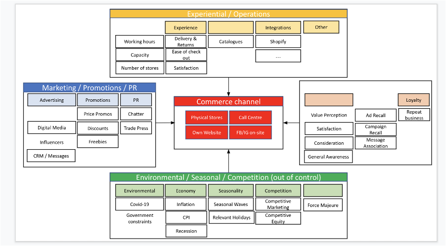
The "demand map"
A demand map is a very helpful practise to identify all relevant factors influencing our business performance. It's strongly recommended to do this exercise, esp. when running MMM for the first time. It's also helpful to revisit your hypothesis regularly.
Variable Transformations
MMM is typlically characterised by the following two hypothesis:
- Ads investment has lagged effect / carries over through time. For example, I see ads today and buy next week.
- Ads investment has diminishing returns. For example, the more I spent on a channel, the less marginal return I will get.
Robyn conducts two types of transformation to account for these hypothesis:
- Adstock transformation
- Saturation transformation
Adstock
Adstock refers to the hypothesis of ads carryover and reflects the theory that the effects of advertising can lag and decay following initial exposure. It's also related to certain brand equity metrics like ad-recall or campaign awareness. The logical narrative is "I saw the ads X days ago before I bought the product". Usually, it's assumed that this "memory" decays as time passes. But there're also cases when it's legitimate to assume that the effect of this "memory" will increase first before decreasing. For example, expensive products like cars or credits are unlikely to be purchased directly after the ads, esp. for offline channels. Therefore, it's usual to assume lagged effect with later peaks for offline channels for these products. At the same time, online conversions from digital channels might be suitable without lagged peaks and only deal with decay.
The formula for adstock can be generalised as:
media_adstocked_i = media_raw_i + decay_rate * media_raw_i-1, where i is a given time period.
There are three adstock transformation options you can choose in Robyn:
Geometric
The one-parametric exponential decay function is used with theta as the fixed-rate decay parameter. For example, an adstock of theta = 0.75 means that 75% of the ads in Period 1 carryover to Period 2. Robyn's implementation of Geometric transformation can be found here and is shown conceptually as followed:
media_adstocked_ij = media_raw_ij + decay_rate_j * media_raw_i-1_j, where i is a given time period and j depicts a media variable. The decay_rate_j is a constant value per media variable and equal to the Geometric parameter theta.
Some rule of thumb estimates we have found from historically building weekly-level models are that TV has tended to have adstock between 0.3 - 0.8, OOH/Print/Radio has had 0.1-0.4, and Digital has had 0.0 - 0.3. This is anecdotal advice so please use your best judgement when building your own models.
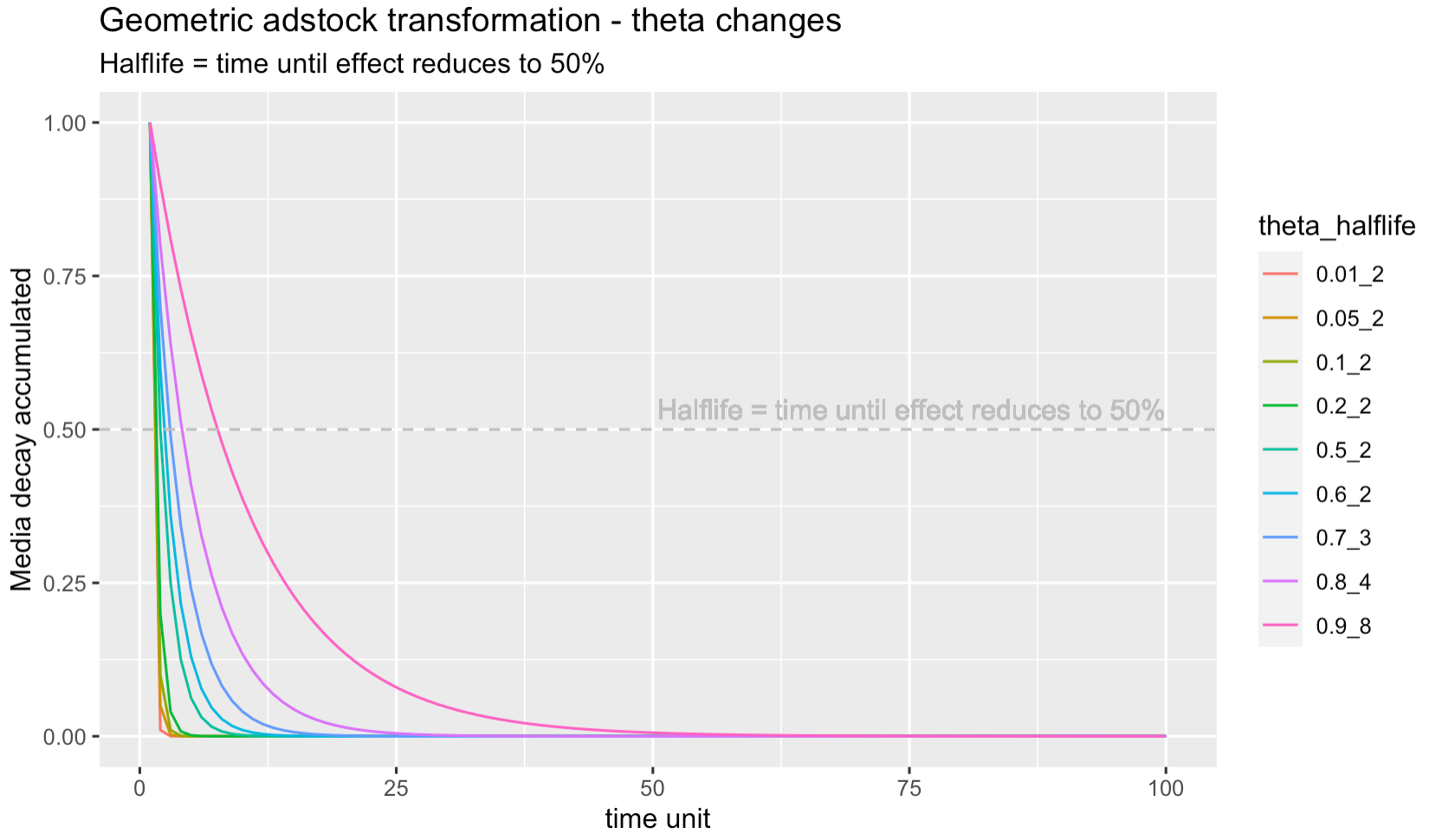
Another useful property of Geometric decay is that the limit of the inifinite sum is equal to 1 / (1 - theta). For example, when theta = 0.75, its infinite sum is 1 / (1 - 0.75) = 4. Because Robyn conducts adstock transformation on spends, it can give you a quick and inituitive idea of how much "inflation" the adstock transformation will add on your raw data. On the other hand, Geometric decay is not able to capture more flexible time-varying decay, nor the lagging effect, which are solved by the Weibull adstock below.
Weibull PDF & CDF
Robyn offers the two-parametric Weibull function in the formats of PDF and CDF. Compared to the one-parametric Geometric function where theta is equal to the fixed decay rate, Weibull produces a vector of time-varying decay rates through more flexibility in the transformation with the parameters shape and scale. Robyn's implementation of Weibull transformation can be found here and is shown conceptually as followed:
media_adstocked_ij = media_raw_ij + decay_rate_ij * media_raw_i-1_j, where i is a given time period and j depicts a media variable. Note that the decay_rate_ij specific to time period i of the media variable j, compared to the fixed decay rate from Geometric.
The plot below shows the flexibility of Weibull adstocks with regard to the two parameters shape and scale. This flexibility does come at a cost of more computational power due to the extra hyperparameters. Weibull PDF is strongly recommmended for products with longer conversion window. We've seen Weibulll PDF leading to considerabaly better fit in some cases.
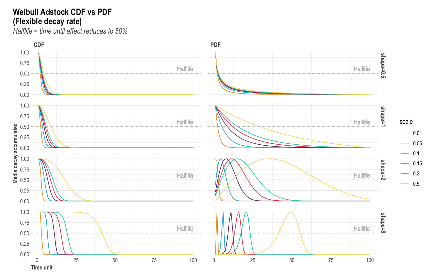
Weibull CDF adstock: The Cumulative Distribution Function of Weibull has two parmeters
shape & scale that enables flexible decay rate, compared to Geometric adstock with fixed
decay rate. The shape parameter controls the curvature of the decay curve. Recommended
bound is c(0.0001, 2). The larger the shape, the more S-form the curve becomes. The smaller
the shape, the more L-form. scale controls the inflexion point of the curve. We recommend
very conservative bounce of c(0, 0.1), because scale increases the adstock half-life greatly.
Weibull PDF adstock: The Probability Density Function of the Weibull also has two
parameters, shape & scale, and also provides flexible decay rate as Weibull CDF. The
difference is that Weibull PDF offers lagged effect. When shape > 2, the curve peaks
after x = 0 and has NULL slope at x = 0, enabling lagged effect and sharper increase and
decrease of adstock, while the scale parameter indicates the limit of the relative
position of the peak at x axis; when 1 < shape < 2, the curve peaks after x = 0 and has
infinite positive slope at x = 0, enabling lagged effect and slower increase and decrease
of adstock, while scale has the same effect as above; when shape = 1, the curve peaks at
x = 0 and reduces to exponential decay, while scale controls the inflexion point; when
0 < shape < 1, the curve peaks at x = 0 and has increasing decay, while scale controls
the inflexion point. When all possible shapes are relevant, we recommend c(0.0001, 10)
as bounds for shape; when only strong lagged effect is of interest, we recommend
c(2.0001, 10) as bound for shape. In all cases, we recommend conservative bound of
c(0, 0.1) for scale. Due to the great flexibility of Weibull PDF, meaning more freedom
in hyperparameter spaces for Nevergrad to explore, it also requires larger iterations
to converge.
Saturation
The theory of diminishing returns (also called saturation) holds that each additional unit of advertising investment increases the response at a declining rate. This hypothesis is implemented as variable transformation in marketing mix models.
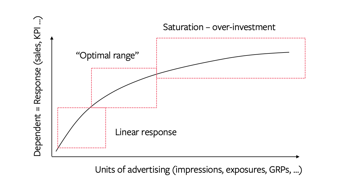
The nonlinear response to a media variable on the dependent variable can be modelled in different ways. Common approaches include transforming the media variable by the logarithm transformation, the power transformation or any sigmoid-shape functions. A common trait of these transformation is that they are all continuous and differentiable, which is important for the budget allocation with any nonlinear optimisation algorithms.
Robyn uses the latter and implements the Hill function for a flexible transformation into S- or L-shape saturation. The implementation of Hill function in Robyn can be found here and is shown conceptually as followed:
media_saturated_j = 1 / (1 + (gamma_j / media_adstocked_j) ^ alpha_j), where
j depicts a media variable.
Note that gamma_j above is scaled to the inflexion point of the variable. By
varying the values of alpha and gamma, changes in curvature and inflexion point
of the saturation curve can be observed below:
In this plot, x axis depicts spend and y response. alpha controls the shape of
the curve between C- and S-shape. Recommended bound for alpha is c(0.5, 3).
The larger the alpha, the more S-shape. The smaller, the more C-shape. gamma
controls the inflexion point of the curve. Recommended bounce of gamma is
c(0.3, 1). The larger the gamma, the later the inflection point in the response
curve.
Another important term that's related to saturation is the marginal response. In mathematical term, the marginal response is equal to the first derivative of a given point at the nonlinear curve. In layman's term, it's the "next dollar response" on a given spend level. For example, if the average weekly spend is 1000$, "what is the return from the 1001th dollar?" This is the foundation of understanding how nonlinear budget allocation works. For more details in marginal response, see this article: "The convergence of marginal ROAS in the budget allocation in Robyn".
Trend & seasonality decomposition with Prophet
As for any real-life time-series problems, it's fundamental to understand trend and seasonality in the data for better fitting. In conventional MMM, this is often done separately and manually using simple assumptions like linear trend or dummy variable for seasonality. With the purpose of reducing human bias in the modeling process, Robyn provides trend, season, holiday & weekday decomposition out of the box using Prophet, a popular time-series forecast package by Meta. In many cases, this has proven to be increasing the model fit greatly. More details on how time-series decomposition works can be found in Prophet's documentaion.
Exemplary time-series decomposition
In the plot below, the dependent variable "revenue" from Robyn's weekly sample data is decomposed into trend, season and holiday components. Note that weekday is not included because it's only available for daily data. Note that the "event" variable is included as an extra regressor. With this, Robyn "converts" a categorical variable to a continuous one, which simplifies later calculation.
Ridge Regression
Marketing Mix Models often encounter the multicollinear issue, because it is a common business practise to operate on different media channels at the same time (e.g. increasing spends on all channels over Christmas). In other words, multicollinearity occurs when more than one independent variables are correlated in a regression model. It results in unstable coefficient estimates, difficulty in interpretation of the coefficient significance as well as overfitting.
Regularised regression is a common choice to counter the challenges of multicollinearity mentioned above. Robyn uses the L2-form of the regularisation, also known as Ridge regression. We've decided for Ridge instead of Lasso (L1-form) regression, because Lasso tends to eliminate features ("zero-out") while Ridge rather reduces their magnitude. For MMM, it's unrealistic to have many media variables having zero effect.
Robyn uses the package glmnet to perform the regularised regression fitting.
The implementation can be found here.
The loss function for Ridge regression is as followed:
The additive model equation is as followed:
A popular question about our model choice is "why not use a Bayesian model". The Bayesian framework has seen rising popularity for business implementations, especially because of many of its attractive properties like the Bayesian prior as a native model calibration feature and the intuitive interpretation of the Bayesian credible interval.
We want to point out that Ridge regression is equivilent to a Bayesian regression with a normal / Gaussian prior, while Lasso corresponds to the Bayesian Laplace prior. This is a well-studied fact academically, for example in the paragraph "Bayesian Interpretation of Ridge Regression and the Lasso" on page 249 in "An Introduction to Statistical Learning" by T.Hastie and co.
Robyn uses an multi-objective algorithm as the optimisation approach,because we believe that the problem a MMM tries to solve has multiple goals. It's often said that MMM is both science and craft. The model is expected to both predict well and "makes sense". From this angle, it's very natural to consider this a multi-objective optimisation problem. Regularised regression has a better fit to our optimizer choice (TwoPointsDE, an evolutionary algorithm from Nevergrad), because the (hyper)parameters are estimated with many evolutionary iterations, as opposed to the typical sampling process with MCMC in a Bayesian regression. More details about multi-objective optimisation and Nevergrad see below.
Multi-Objective Hyperparameter Optimization with Nevergrad
Every MMM practitioner knows this "sanity check": When facing multiple model candidates, it's common to prefer a model that's more "plausible", meaning one with slightly less fit but better alignment with current spend allocation. For example, for a dataset with 2 channels splitting 90%/10% media spend, a model that produces the contribution of 10%/90% is considered rather implausible, no matter how good the model fit is. In comparison, another model with 70%/30% contribution split would be considered more pausible.
In other words, a good MMM needs to be both predictive and interpretable. This is the frequently cited conflict of science and craft. At team Robyn, we considered this a multi-objective optimisation problem, because the reality is never simply prediction. We believe it's important to include the "sanity check" into the optimisation through parameterization in the form of extra objective functions. The implementation of multi-objective hyperparameter optimization is considered the most important innovation in Robyn. At the same time, the usage of hyperparameters enables stronger automation of the parameter selection for adstocking, saturation, regularization penalty and even training size of time-series validation.
Robyn uses Nevergrad, Meta’s gradient-free optimization platform to perform this task with its so-called "ask & tell"" interface. Simply explained, Robyn "asks" Nevergrad for the mutating hyperparameter values by "telling" it which values have better scores (objective functions).
Objective Functions
Robyn implements three objective functions as the "goals" for hyperparameter optimisation currently.
- NRMSE: The Normalized Root Mean Square Error is also referred to as the prediction error. Robyn allows time-series validation with the spitting of the dataset into train / validation / test. When fitting without the time-series validation, the training error
nrmse_trainis objective function for the evolving iterations. With time-series validation, the validation errornrmse_valbecomes the objective function, whilenrmse_testis used to assess the out-of-sample preditive performance. - DECOMP.RSSD: The Decomposition Root Sum of Squared Distance is also referred to as the business error and is a key invention of Robyn. It represents the difference between share of spend and share of effect for paid media variables. We're aware that this metric is controvertial because of the convergence of media ROAS. In the reality, multiple objectives always "work together" and trade off each other in the optimisation process. DECOMP.RSSD rules out models with extreme decomposition and helps narrowing down model selection.
- MAPE.LIFT: The Mean Absolute Percentage Error for experiments is activated when calibrating and is referred to as the calibration error. It's a key invention of Robyn and allows Robyn to minimise the difference between predicted effect and causal effect.
Hyperparameters
There're four types of hyperparameters in Robyn at the moment.
- Adstocking:
thetawhen selecting Geometric adstocking, orshape&scalewhen selecting Weibull adstocking - Saturation:
alpha&gammafor Hill function - Regularization:
lambdafor the penalty term in ridge regression - Validation:
train_sizefor the percentage of training data
The cardinality of hyperparameters increases when adding more paid and organic media variables, because Robyn performs adstocking & saturation transformation for each media variable individually. For example, if using 10 media variables with Geometric adstock, the total amount of hyperparameters is 32: 10 thetas + 10 alphas + 10 gammas + 1 lambda + 1 train_size. With Weibull adstock, it's 42: 10 shapes + 10 scales + 10 alphas + 10 gammas + 1 lambda + 1 train_size. Adding hyperparameters will give Robyn more flexibility to find optimum solutions, but it will trade-off model runtime because it needs longer to converge.
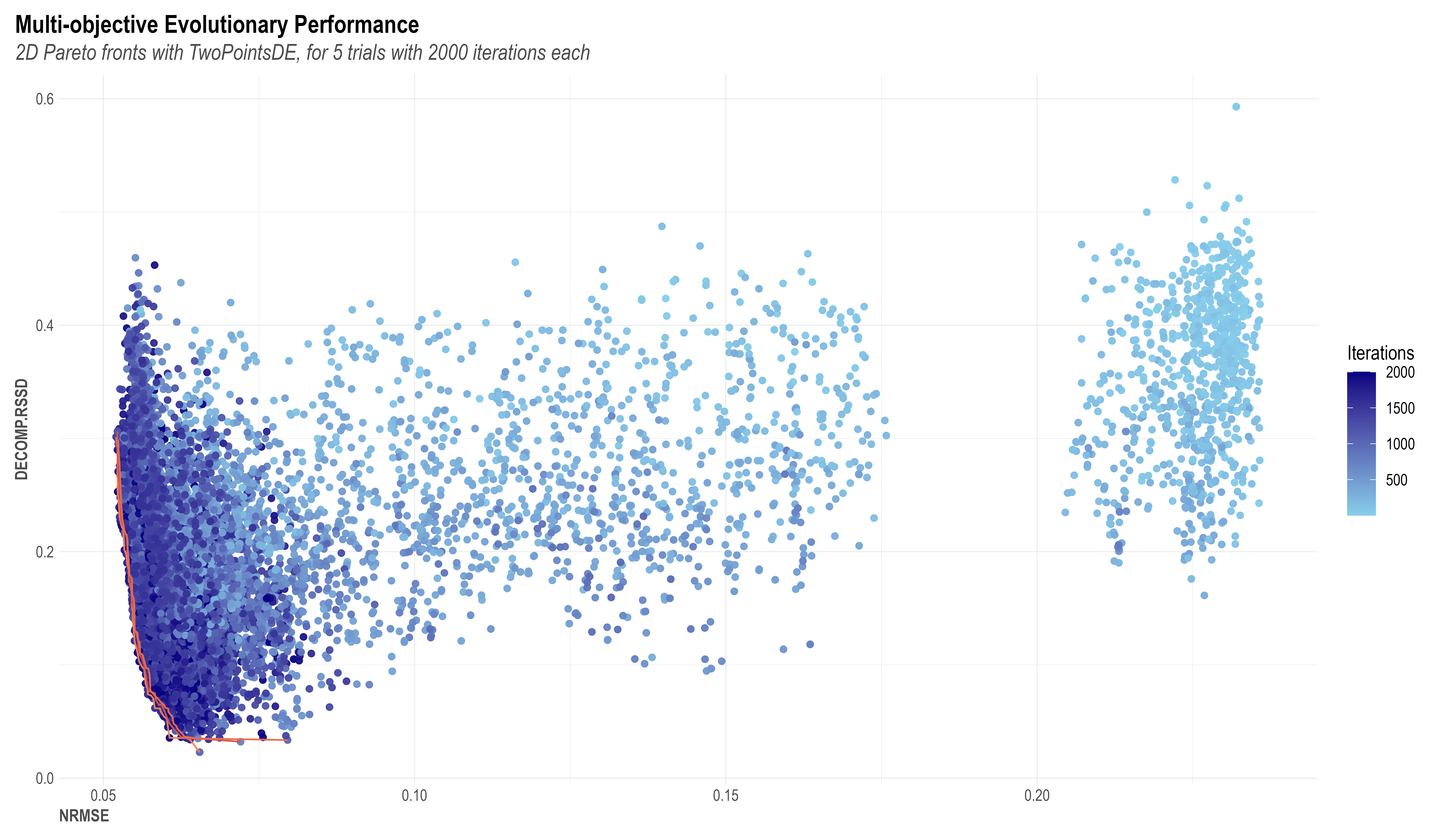
Using the concept of Pareto-optimality balancing all objective functions, Robyn always outputs a set of pareto-optimum model candidates that are considered "the best". Please find below an example of an example chart of the Pareto model solutions. Each dot in the chart represents an explored model solution, while the lower-left corner lines are Pareto-fronts 1-3 and contains the best possible model results from all iterations. The two axes (NRMSE on x and DECOMP.RSSD on y) are the two objective functions to be minimized. As the iteration increases, a trend down the lower-left corner of the coordinate can be clearly observed. This is a proof of Nevergrad's ability to drive the model result towards an optimal direction.
The premise of an evolutionary algorithm is that of natural selection. In an evolutionary algorithm you may have a set of iterations where some combinations of coefficients that will be explored by the model will survive and proliferate, while unfit models will die off and not contribute to the gene pool of further generations, much like in natural selection. In robyn, we recommend a minimum of 2000 iterations where each of these will provide feedback to its upcoming generation, and therefore guide the model towards the optimal coefficient values for alphas, gammas and thetas. We also recommend a minimum of 5 trials which are a set of independent initiations of the model that will each of them have the number of iterations you set under ‘set_iter’ object. E.g. 2000 iterations on set_iter x 5 trials = 10000 different iterations and possible model solutions.
In Robyn, we consider the model to be converged UNDER REVISION when:
Criteria #1: Last quantile's standard deviation < first 3 quantiles' mean standard deviation
Criteria #2: Last quantile's absolute median < absolute first quantile's absolute median - 2 * first 3 quantiles' mean standard deviation
The quantiles are ordered by the iterations of the model, so if we ran 1000 iterations, the first 200 iterations would make up the first quantile. These two criteria represent an effort to demonstrate that both the standard deviation and the mean for both NRMSE and DECOMP.RSSD have improved relative to where they began, and they are not as variable.
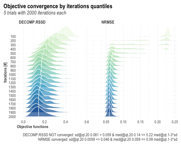
Alternatively, run the following code to observe the convergence of your multi-objective optimization in the ridgeline visualization.
OutputModels$convergence$moo_distrb_plot
Time Series Validation
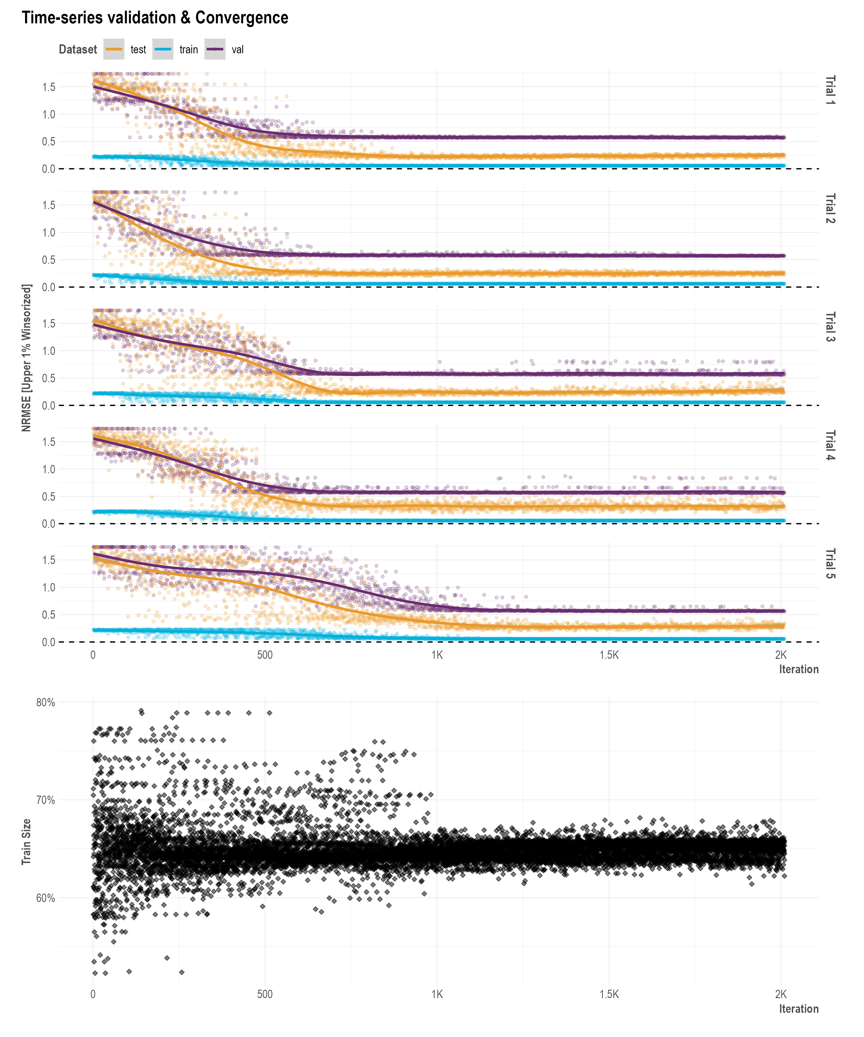
When ts_validation = TRUE in robyn_run() a 3-way-split time series for NRMSE validation is enabled.
A time series validation parameter train_size is included as one of Robyn's hyperparameters. When ts_validation = TRUE in robyn_run(), train_size defines the percentage of data used for training, validation and out-of-sample testing. For example, when train_size = 0.7, val_size and test_size will be 0.15 each. This hyperparameter is customizable or can be fixed with a default range of c(0.5, 0.8) and must be between c(0.1, 1).
Model Clustering
As depicted in plot 4 in session model onepager below, the k-means clustering is used to further reduce model choice. Robyn uses bootstrapping to calculate uncertainty of ROAS or CPA.
- Use k-means clustering on all pareto-optimal model candidates to find clusters of models with similar hyperparameters. The constant k describes the number of clusters.
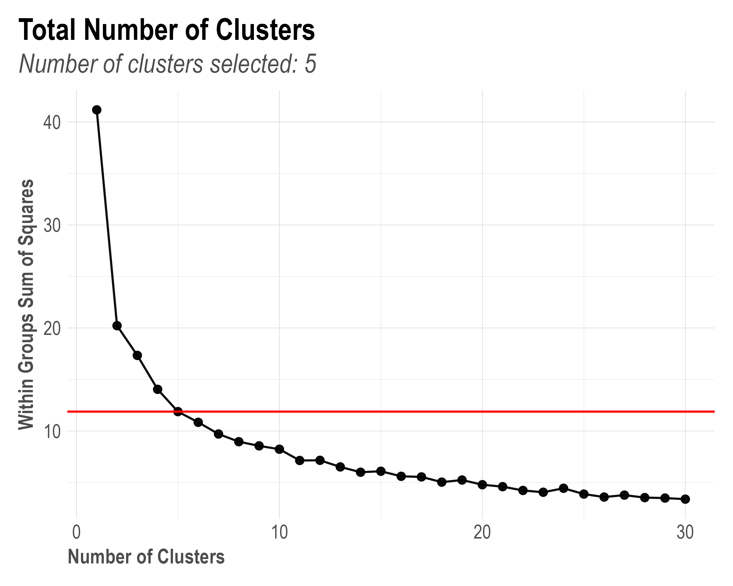
- When
k = "auto"(default value), WSS (Within Group Sum of Squares) is calculated to automatically find the best k value between 1-20. The k value with <5% WSS change from the previous k is selected. This is visualised in the screenshot below. - Within each of the k clusters, a winner model is selected based on the three normalised objective functions (NRMSE, DECOM.RSSD, and MAPE if calibrated was used).
- In the context of MOO, we consider each cluster a sub-population in a different local optimum.
Calibration of average effect size with causal experiments
Randomised controlled trial (RCT) is an established academic gold standard to infer causality in science. By applying results from RCT in ads measurement that are considered ground truth, you can introduce causality into your marketing mix models. Robyn implements the MMM calibration as an objective function in the multi-objective optimization by parameterizing the difference between causal results and predicted media contribution.
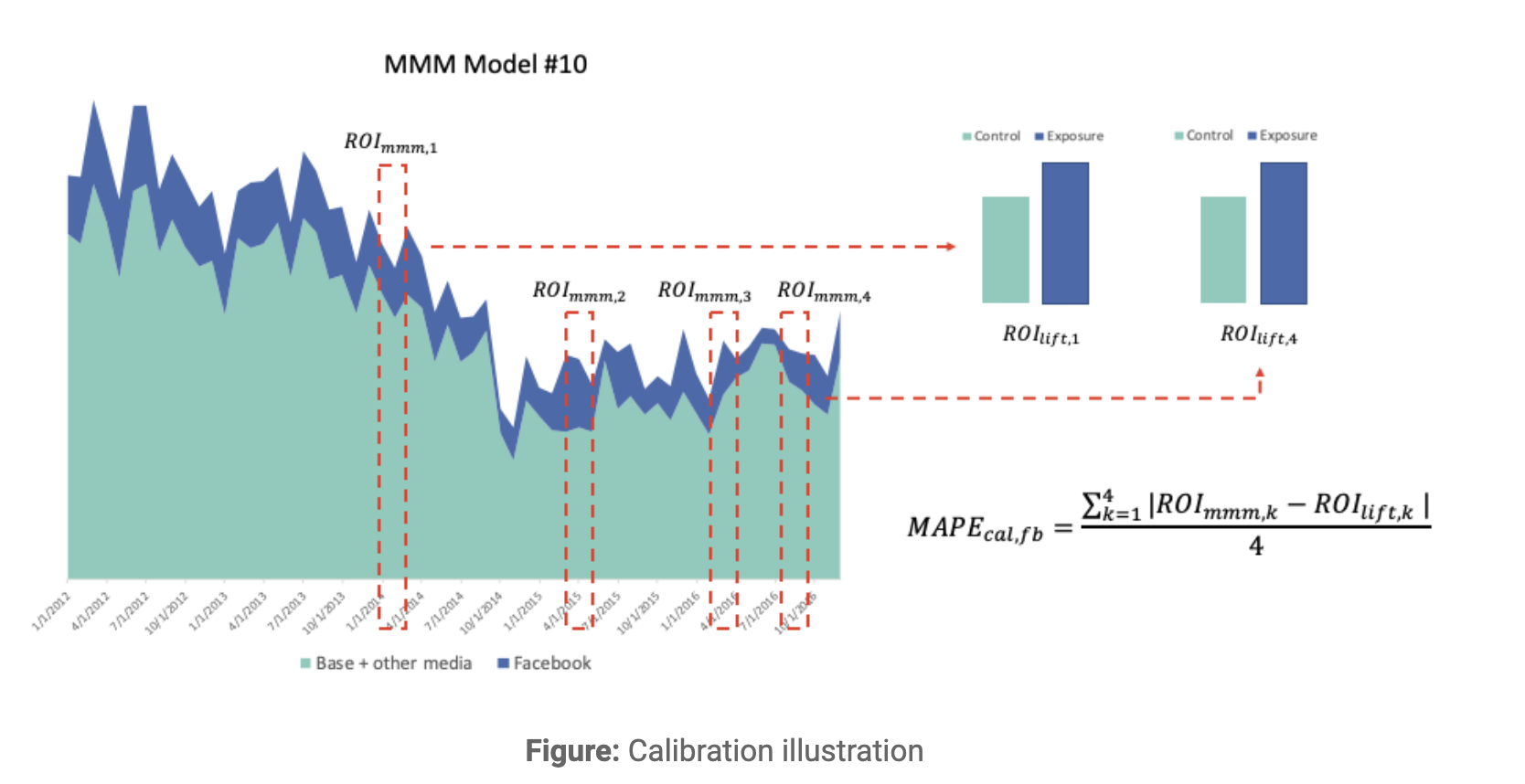
The chart above illustrates the calibration concept. The calibration error MAPE.LIFT is implemented as the third objective function besides the prediction error and the business error (please refer to details above) and depicts the difference between predicted media contribution and the ground truth, as shown in the equation in the chart.
Key findings of calibration
- According to an third party whitepaper "The Value of Calibrating MMM with Lift Experiments" by Analytic Edge, uncalibrated models show 25% average difference to the ground truth.
- Another simulated experiment conducted by the the winners of the Robyn 2022 Hackathon has found out that:
- Calibrated models are better: All calibrated models show predicted ROAS closer to true ROAS with smaller MAPE than uncalibrated models.
- Good for one, good for all: When only calibrating one from both simulated channels (TV & FB), the other channel also predicts better towards true ROAS than uncalibrated.
- The more calibrated channels, the better: Calibrating both simulated channels (TV & FB) shows the lowest error to true ROAS. This is expected, because Robyn’s calibration is designed to recover the true ROAS by having the calibration error (MAPE.LIFT) as an objective function within Robyn’s multi-objective optimisation capacity.
- The more studies to calibrate, the better: The true ROAS prediction improves strongly with up-to 10 studies per channel.
Types of experiments
There're two major types of experiements in ads measurement, as pointed out by this WARC article "A step-by-step guide to calibrating marketing mix models with experiments".
- Sales experiments: These experiments aim to measure the impact of marketing activities on sales such as online conversion. Examples are Meta’s Conversion Lift or Google’s Conversion Lift. These experiments work by comparing the conversion rates between a test group and a control group, and help estimate the causal effect of marketing.
- Pros: Provide direct insight into sales impact, relatively straightforward to plan and execute.
- Cons: Limited to measuring conversion-related outcomes, may overlook non-conversion effects. Only applicable to digital channels.
- Geo experiments: Geo experiments analyze the impact of marketing activities in specific geographic regions such as DMAs, states or cities. By comparing the outcomes in regions exposed to marketing interventions with those in control regions, the spatial variation in response can be quantified.
- Pros: Capture spatial variations and market-specific responses, useful for localized marketing. Possibility to run offline. Same test for cross channel. Can estimate groups of channels (e.g. all digital). Might even be applicable for offline channels like addressable TV or OOH.
- Cons: Could get affected by potential spillover effects across regions, requiring careful design to ensure comparability.
Robyn accepts a dataframe as calibration input in the robyn_inputs() function. The function usage can be found in the demo.
Holistic calibration
Rethinking calibration
The triangulation of MMM, experiments and attribution is the centerpiece of modern measurement. While there's no universally accepted definition of calibration, it often refers to the adjustment of estimated impact of media between different measurement solutions.
In MMM, calibration usually refers to adjusting the average effect size of a certain channel by causal experiments, as explained in details above. However, the average effect size, or the beta coefficient in a regression model, is not the only estimate in an MMM system. The bare minimum of a set of estimates in MMM includes the average effect size, adstock and saturation. And just as the effect size, adstock and saturation are uncertain parametric quantities that can and should be calibrated by ground truth whenever possible. We believe that holistic calibration is the next step of triangulation and integrated marketing measurement system.
The curve calibrator (beta)
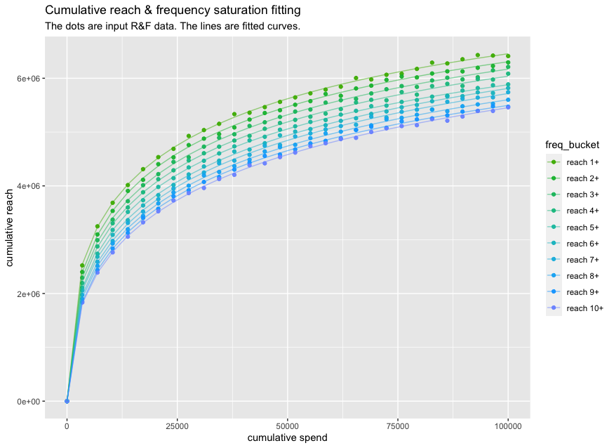
Robyn is releasing a new feature "the curve calibrator" robyn_calibrate() as a step towards holistic calibration. The first use case is to calibrate the response saturation curve using cumulative reach and frequency data as input. This type of data is usually available as siloed media reports for most offline and online channels. The latest choice of reach and frequency data is Project Halo, an industry-wide collaboration that aims to deliver privacy-safe and always-on cross-channel reach deduplication. The above graphic is derived and simulated based on a real Halo dataset with cumulative spend and cumulative reach by frequency buckets. For example, "reach 3+" means reaching 3 impressions on average per person. There's certainly a gap between saturation of reach and business outcome (purchase, sales etc.). However, they're also interconnected along the same conversion funnel (upper funnel -> lower funnel), while the reach & frequency saturation curve is often more available. Therefore, we're exploring the potential of using reach & frequency to guide response saturation estimation.
According to a recent research paper from the Wharton School and the London Business School by Dew, Padilla and Shchetkina, a common MMM cannot reliably identify saturation parameters, quote "as practitioners attempt to capture increasingly complex effects in MMMs, like nonlinearities and dynamics, our results suggest caution is warranted: the simple data used for building such models often cannot uniquely identify such complexity." In other words, saturation should be calibrated by ground truth whenever possible.
Our approach for saturation calibration by reach & frequency: Assuming an extreme situation where every user sees the first impression and purchases immediately. In such a case, response saturation curve equals the reach 1+ saturation curve. Hill function is a popular choice for saturation transformation and implemented in Robyn, where gamma controls the latitude of the inflexion point. A lower gamma means earlier and faster saturation at a lower spend level. Our hypothesis is that the cumulative reach 1+ curve represents the earliest inflexion and thus serves as a reasonable lower boundary for gamma for a selected channel. As frequency increases, the reach inflexion point delays and approaches lower-funnel. We believe that the hidden true response curve lies within the spectrum of cumulative reach and frequency curves. In the dummy dataset, we've simulated reach 10+ to represent the upper bound for gamma. The "best converting frequency" varies strongly across verticals. We believe that reach & frequency it's one step closer to identifying the true saturation relationship. Use domain expertise to further narrow down or widen the bounds. For alpha, we recommend to keeping the value flexible as in default.
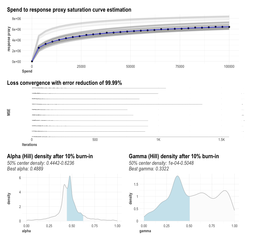
The below graphic is an exemplary visualisation of a curve fitting process, where Nevergrad is used to estimate alpha, gamma as well as the beta. Note that the distribution of alpha and gamma are often multimodal and non-normal, because they rather reflect the hyperparameter optimization path of Nevergrad than their underlying distribution.
To try out robyn_calibrate(), please see this tutorial in the demo.
library(Robyn)
data("df_curve_reach_freq")

# Using reach saturation as proxy
curve_out <- robyn_calibrate(
  df_curve = df_curve_reach_freq,
  curve_type = "saturation_reach_hill"
)
# For the simulated reach and frequency dataset, it's recommended to use
# "reach 1+" for gamma lower bound and "reach 10+" for gamma upper bound
facebook_I_gammas <- c(
  curve_out[["curve_collect"]][["reach 1+"]][["hill"]][["gamma_best"]],
  curve_out[["curve_collect"]][["reach 10+"]][["hill"]][["gamma_best"]])
print(facebook_I_gammas)
Customizable for 3rd-party MMM
While the curve calibrator is released within the Robyn package, it can be used as a standalone feature without having built a model in Robyn. The current beta version is piloting the two-parametric Hill function for saturation. Any MMM solution, not only Robyn, that employs the two-parametric Hill function can be calibrated by the curve calibrator.
In the future, we're planning to partner with our community, advertisers, agencies and measurement vendors to further explore this area and also to expand the curve calibrator to cover other popular nonlinear functions for saturation (e.g. exponential, arctan or power function) as well as adstock (geometric or weibull function).
Model onepager
Robyn automatically exports various graphical and tabular outputs into the specified path to aid result interpretation and further custom analysis. An onepager per pareto-optimal model is exported after running the robyn_outputs() function. An example:
Response decomposition waterfall: This chart depicts the absolute as well as percentage contribution of all of independent variables. The percentages sum up to 100% and can be interpreted as "x% of the revenue can be explained by variable A". The concept "baseline" might come up in the context of total decomposition. While there's no clear definition of baseline, we define baseline as "non-steerable variables". All marketing-related variables (paid, organic, price, promotion etc.) are considered steerable. The rest of seasonal (trend, season, holiday etc.), external variables (competitors, weather etc.) and intercept are considered baseline.
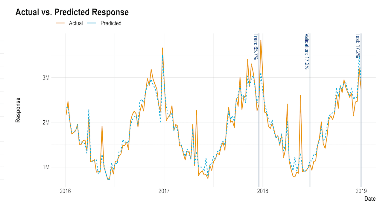
Actual vs. predicted response: This chart shows the actual response variable (e.g. revenue) vs. the predicted value from the model. The goodness of fit can be observed visually. In this example, the R-squared is considerably high (close to 0.9), while both actual and predicted lines are visually well aligned. Moreover, this plot helps the interpretation of "unmatched events", e.g. the peak mid 2018 is not captured by the model at all. Was there a special event that's not accounted for in the model?
Share of spend vs. share of effect: This plot shows the comparison between the total effect share and total spend share for all paid media variables within the entire modeling window. This is the visualization of the objective function DECOMP.RSSD. Moreover, the total return on investment (ROAS) of each media variable are also plotted. Note that the percentage of effect will sum up to 100% for media variable only in this plot, as opposed to the waterfall plot that contains all variabes.
In-cluster bootstrapped confidence interval: Robyn uses bootstrapping to calculate uncertainty of ROAS or CPA. After obtaining all pareto-optimal model candidates, the K-means clustering is applied to find clusters of models with similar hyperparameters. In the context of MOO, we consider these clusters sub-population in different local optima. Then we bootstrap the efficiency metrics (ROAS or CPA) to obtain the distribution and the 95% interval.
Adstock decay rate: This chart represents the carryover effect of each media variable (paid & organic). For Geometric adstock, the barchart depicts the fixed decay rate. The higher the value, the stronger the carryover into the future. For Weibull adstock, each sub-chart depicts the time-varying decay rate for each media variable, which might also include lag effect. A common hypothesis of adstock is that offline channels have stronger the carryover.
Immediate vs. carryover: Robyn splits the media contribution into two parts: immediate contribution and carryover contribution. Immediate is the effect of the direct media spend of a given period, while carryover is the effect of historical spend "leaked" (also called adstock) into the given period. Conceptually, the carryover effect can be understood as the effect of upper-/mid-funnel brand equity metrics like "ad recall" or "campaign awareness". Note that we avoid using the terms "short-term" and "long-term", because we believe, without any agreed definition, that the "long-term effect" should describe media impact on baseline sales. In comparison, adstocking only addresses media's direct impact on the response and says nothing about the interaction with baseline. Note that it's possible to have a channel with higher carryover but lower adstock, as seen in this example above with
ooh_Svstv_S. The reason lies in the different saturation curves per media (explained below) that also have impact on the carryover decomposition.Saturation curves: Saturation curve has many synonyms, like response curve or diminishing return. Robyn calculates one saturation curve (one set of Hill parameters) per media variable. The grey area depicts the historical carryover, as explained in point 6 above: The end of grey area projected on the Y-axis is the carryover effect, while the dot (average spend) projected on Y is the total effect. The difference between these two is the immediate effect. Use your business context to make sense of these curves. For example, an over-spending media variable would expect the dot on the flatter area of the curve, representing lower marginal ROAS or mROAS, the most important metric for budget allocation. For more details see this article "The convergence of marginal ROAS in the budget allocation in Robyn". Tip: You can also use the
robyn_response()function in to recreate these response curves. For details see the demo.Fitted vs. residual: This chart shows the relationship between fitted and residual values. For a good fitting model, this plot is expected to show rather horizontal trend line with the dots evenly scattered around the X-axis. On the contrary, visible patterns (funnle shape, waves, groupped outliers) indicate missing variable in the model.
Budget allocation
Robyn's budget allocator comes with two scenarios:
- Maximum response: Given a total budget and media-level constraints, the allocator calculates the optimum cross-media budget split by maximising the response. For example: "What's the optimum media split if I have budget X?"
- Target efficiency (ROAS or CPA): Given a target ROAS or CPA and media-level constraints, the allocator calculates the optimum cross-media budget split and the total budget by maximising the response. For example: "What's the optimum media split and how much budget do I need if I have want to hit ROAS X?"
Robyn uses the optimisation package “nloptr” to perform the gradient-based nonlinear optimisation with bounds and equality constraints. Augmented Lagrangian (AUGLAG) is used for global optimisation and Sequential Least Square Quadratic Programming (SLSQP) for local optimisation. For algorithmic details please see nloptr’s documentation.
Below is an example allocator onepager:
For the interpretation of the budget allocation onepager, please refer to the following deepdive articles:
- "The convergence of marginal ROAS in the budget allocation in Robyn": here
- "Hitting ROAS target using Robyn’s budget allocator": here
The reach & frequency allocator (prototype)
Reach and frequency planning is conducted frequently by advertisers and media agencies. To further harvest the power of Project Halo and provide more actionability for R&F data, we're experimenting on a new feature "reach and frequency allocator". It answers the question “what’s the optimal combination of reach & frequency” on a channel given a total budget and average CPM. It consumes the saturation information from R&F data and uses nonlinear optimization to find the optimal point with highest response.
Decription of the graphic below: Given 100k budget and 6$ CPM, as well as the estimated saturation curve for reach and frequency separately using Halo data, the optimum R&F combination is 5.67M reach x 2.94 frequency, with the maximum response (sales) of 317.8k$.
It's currently a prototype and not yet available. An MVP is expected in 2025.
Model refresh
Conventionally, the model refresh cycle of MMM is bi-annual or even longer. The time delay leads to limited actionability of MMM insights. Robyn's model refresh feature aims to solve this challenge and enables model refresh and reporting as frequently as the data allows. It also enables MMM to be a continuous reporting tool for actionable and timely decision-making that could feed your reporting or BI tools.
Conceptually, the model refresh function robyn_refresh() builds on top of an selected initial model, updates its hyperparameter with a narrower range that's proportional to the new data / total data ratio and picts an winning model based on the combination of objective functions. Note that model refreshing comes with certain common expectations. When refreshing with a shorter period of new data, it's expected:
- that the refreshed model has stable baseline compared to initial model
- that the refreshed model reflects the media spend changes in the new period
Robyn uses modified objective functions to achieve the above. To be precise, the NRMSE only accounts for the new period while refreshing, because the main goal of refreshing is to better describe the new period. The DECOMP.RSSD is modified to drive only effect share closer to the refresh spend share, while it also accounts for the similarity between new and old baseline.
The example below shows the model refreshing mechanism for 5 different periods of time based in an initial window covering most of 2017 and 2018:
The second refresh chart shows the model decomposition across initial and various refresh models:
Note that this feature is not yet tested thoroughly and might provide instable refresh results.